Thermodynamic Bounds and an Optimal Tempo for Goal-Holding Agents
A definition of an agent with an energy budget, the physical bounds on how fast such an agent can act per second and per joule, and a reading of intelligence as progress per joule on a completed run.
David Charlot, Open Interface Engineering
Research studies, not journal finals. Notation is defined in the paper. Analytical energy estimates are not board power. Interactive figures live under /living/. Shared terms: glossary.
Cite this
Genre: Research paper · definition, kinematic bounds, calculus
David Charlot, Open Interface Engineering. Thermodynamic Bounds and an Optimal Tempo for Goal-Holding Agents. Open Interface Engineering. Web: https://research.openie.dev/papers/agency/. PDF: https://research.openie.dev/pdfs/agency.pdf.
Thermodynamic Bounds and an Optimal Tempo for Goal-Holding Agents
Version 1.1, 11 October 2026. Data and code: research.openie.dev/data/. LaTeX PDF: /pdfs/latex/agency.pdf (source).
Abstract
This paper defines an agent as a system that holds a goal under an energy budget, derives physical limits on how fast it can act per second and per joule, and measures intelligence as progress per joule after a run is complete.
In plain words
- To count as an agent, a system must aim at a goal, act on the world, and stay within an energy budget.
- Physics sets a minimum energy cost for every decision, so no agent can act faster or cheaper than that limit.
- Among systems that get the job done correctly, the smarter one is the one that used less energy.
1. Thesis
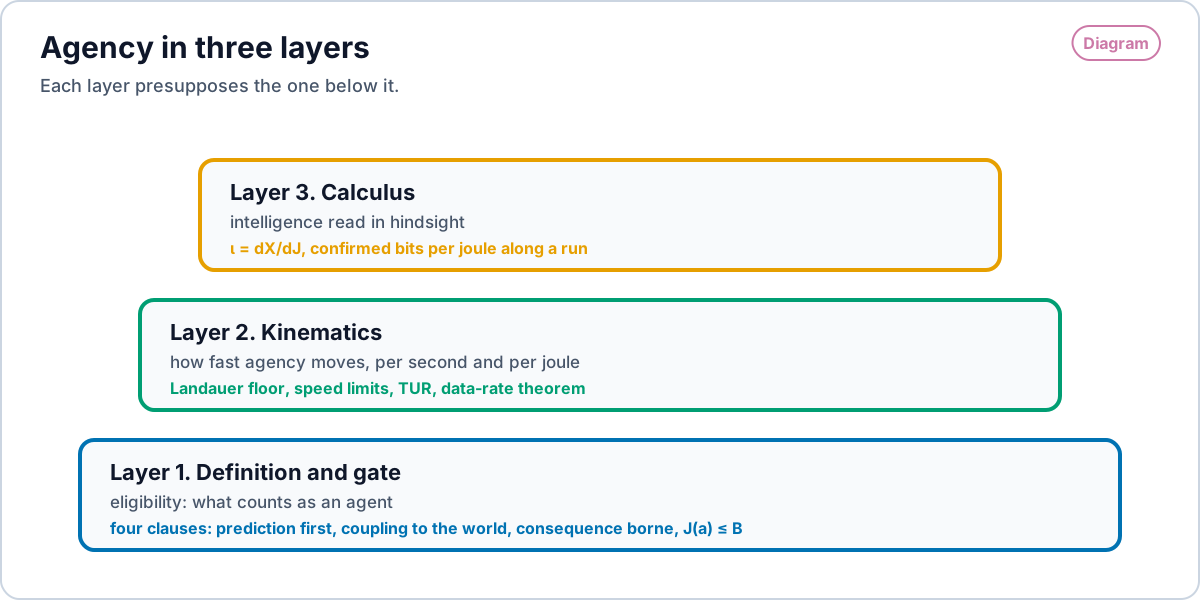
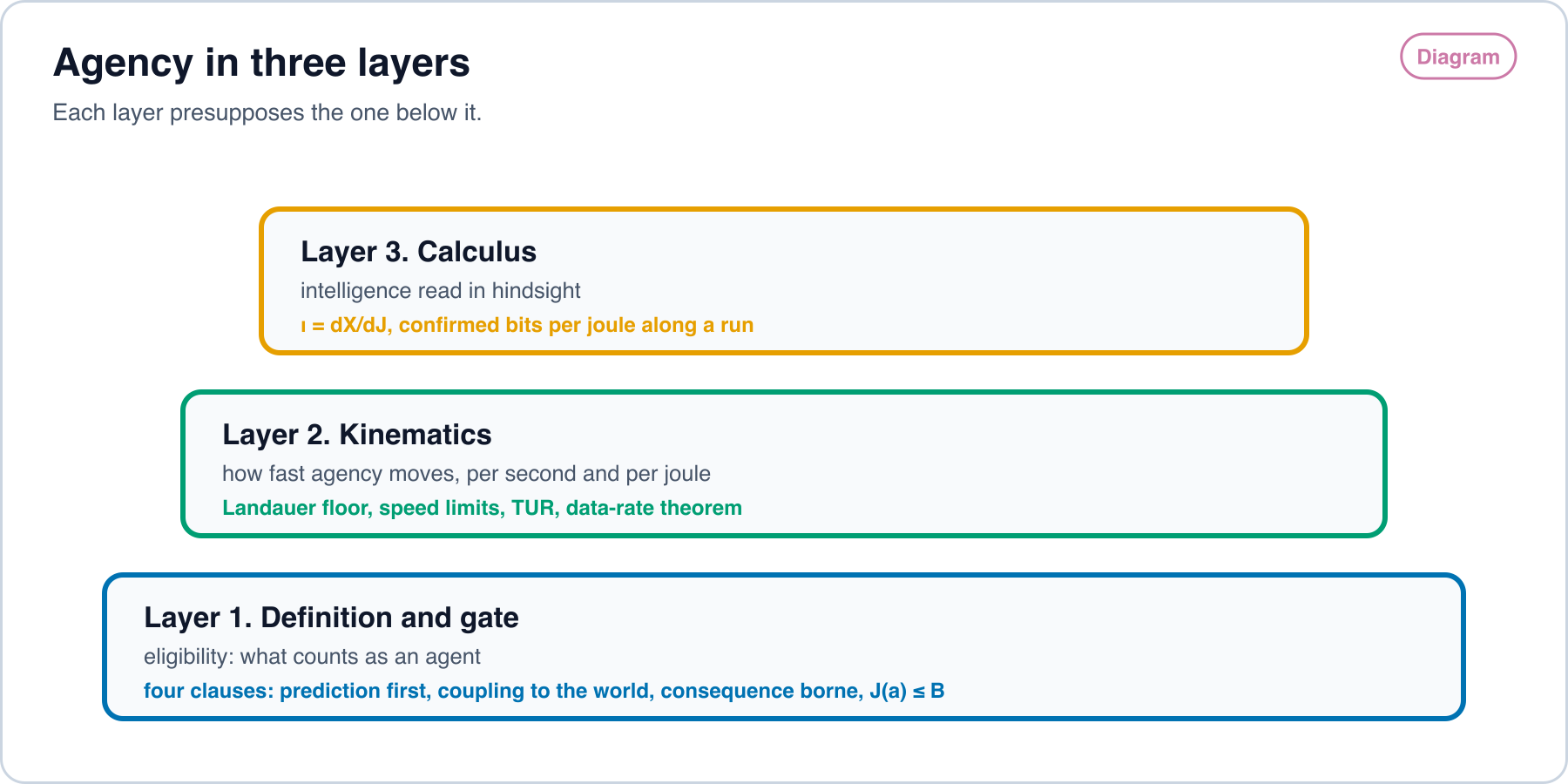
The proposal has three layers, and the order is fixed.
- Agency comes first, and its definition is required. This track proposes it as the Universal Law of Agency. In form it is a definition plus a gate: four clauses say what counts as an agent, and the fourth clause refuses any act that breaks the joule budget. Nothing is an agent until the definition is met. Nothing downstream is defined without it.
- The kinematic bounds of agency follow from the definition. They say how fast agency can move, per second and per joule, and what it must pay to move.
- Intelligence is the calculus of agency. Intelligence is a hindsight characteristic. It is read off a completed run, the way velocity is read off a recorded path. It is therefore a derivative of agency: , where is confirmed agency and is joules.
The thesis: among systems that pass a task’s correctness test, the ranking is by energy to completion, in joules.
The thesis is read through its gate. Capability is not discarded: it is the gate. Burnell and colleagues ask that evaluation report results by instance rather than one aggregate [333], and Zhou and colleagues and Laber and colleagues find that capability and efficiency vary independently across models and inference budgets [334, 335]. Those findings are about systems that do not all pass the same predicate. Once a predicate and a failure rate are fixed, every factor other than joules has already been spent in passing the gate, and that is the sense of the thesis’ second sentence. The gated ranking is also practice: SPECpower ranks server work per watt at stated load [338], cost-of-pass ranks models by the cost of a correct answer [336], and intelligence per watt ranks local models by accuracy per unit power [337]. This paper’s contribution is the joule form of that ranking with a refusal clause and a hindsight derivative, not the idea of ranking by cost under correctness.
The gate and the ranking separate two things that are often merged: capability and intelligence. Capability is passing at all. Intelligence is how few joules the pass takes. Krakauer, Mitchell and Krakauer draw the same line from complexity science: impressive capabilities are not mistaken for intelligence, which is reserved for solving problems “quickly and parsimoniously, with a minimal expenditure of energy” [339]. Two systems that hand over the same correct answer, one directly and one after a long detour, are equally capable. Only the first is the more intelligent, and is the quantity that tells them apart. A system can be made more capable by spending more. It is made more intelligent only by spending less for the same pass.
The thesis has an exact form. Correctness is a gate. Joules are the ranking. For a task with completeness predicate , the joules to correct completion of system are
The minimum runs over the policies that can execute, and is the failure rate the task allows. A deadline, when the task has one, is written into : an answer after its deadline fails the predicate. So correctness, deadlines and task size appear in the formulas of this track, and each appears as a constraint. None appears as a score. Among systems that pass the gate, joules alone order them. Parameters, tokens, benchmark scores and prices carry zero weight in that order. That is what “collapse to zero” means. Correctness becomes the constraint, and energy becomes the only metric. That is the thesis. Energy-to-solution in high-performance computing and the accuracy-gated measurements of MLPerf Power have the same form [260]. This track puts an eligibility definition in front of the gate and reads the joules as a metered density. Section 2.3 states the ranking. Proposition 8 proves that it is a total order on systems that survives bounded meter error, and that integrated is not.
The order matters. A derivative needs a path. A path needs something that moves. The definition says what moves. The kinematics say how it can move. Intelligence is read off the path afterward.
This track tests that order against the literature. It sorts every source into three bins.
- Proven: theorems and derivations. The result follows from stated assumptions.
- Demonstrated: experiments, measurements and simulations. The result was observed.
- Opinion: position papers, frameworks, definitions and philosophy. The result is argued.
No source is excluded for its method. Each source is placed by what it gives the definition, the kinematics or the calculus.
Terms
- SI: the International System of Units.
- Joule (J): the SI unit of energy. One watt for one second.
- : the Boltzmann constant, J/K, exact by SI definition.
- Entropy production (): the total entropy a process creates, in units of . It is zero only for a reversible process.
- Mutual information (): the number of bits one variable carries about another.
- Dynamical activity (): the rate of jumps between states in a stochastic process. It measures how busy the dynamics are.
- TUR (thermodynamic uncertainty relation): a theorem that ties the precision of a current to its entropy production.
- NMR (nuclear magnetic resonance): a method that controls and reads molecular spins.
- Instability rate (): how fast an uncontrolled world drifts from the goal, in nats per second. For a linear plant run at steps per second, .
- Reset error (): the probability that a reset record is not in its most likely state.
- Counting observable: a quantity of a trajectory that counts selected jumps. It never decreases.
- Radon-Nikodym derivative: the density of one measure with respect to another. It exists when the first measure gives zero mass to every set that the second gives zero mass to.
- Mixture of Limits: the rule of using the cheapest mechanism (gear) that is sufficient. There exist floors past which additional tokens, parameters, or joules do not purchase verifiable progress. Spend past the floor is waste. That floor is the plateau (threshold convergence). Mixture of Limits is not one fixed cascade. A fixed cascade order is one instance of it. The σ-law selector is another.
- Receipt: a record attached to every act, holding its prediction, its outcome and its joules.
2. Formal framework
Definitions fix the terms. Propositions are proven from cited theorems, with their assumptions stated.
Figure 1 shows how the three layers stack.
2.1 Layer 1. The definition and its gate: eligibility
For a system , an act and an episode budget in joules, eligibility equals 1 only when all four clauses hold.
- Prediction first. A result template is fixed at time , before the act, and it discriminates: . Here is the probability that the template rejects an outcome drawn without the act, and is fixed with the template. A template that accepts every outcome predicts nothing.
- Coupling to the world. . Here is the world state downstream of the actuator, and is Pearl’s intervention operator [1]. The coupling must survive changes to the system’s own inputs. Editing your own sensors does not count [2].
- Consequence borne. The comparison (match, partial, mismatch) changes the system: .
- Physical floor: the joule budget. . If no act meets clauses 1 to 4, the act is refusal, with a receipt.
Physics already prices clauses 1 to 3. The second law with feedback [3, 4] and the measurement and erasure bound [5] give, for one bath at temperature :
Here is the mutual information the act’s comparison acquires, in nats. One bit is nats, so each bit costs . An acceptor that compares and then resets pays at least per bit over a closed cycle [6, 7]. The definition is physical from its first clause.
Definition 1. Coupling
Clause 2 is measured by causal information flow. Let act be drawn from the policy and set by intervention, and let be the world downstream of the actuator. Then
This is the information flow of Ay and Polani from the act node to [8]. It equals the mutual information of the interventional joint distribution . Its maximum over policies is the capacity of the channel from acts to the world:
Here is the set of available acts. Klyubin, Polani and Nehaniv defined empowerment as this capacity, with the agent’s own future sensors in place of [9]. Clause 2 takes the world side, so editing a sensor adds nothing [2].
Realized, not capacity. The quantity credited to an act is the realized flow under the policy the agent ran: at that . The capacity is an upper bound and is never credited. A system is not credited for coupling it could have made and did not.
Estimation. The flow is estimated from receipts. The agent’s randomized policy assigns acts, so the receipt’s joint counts of are interventional samples. The plug-in mutual information of those counts is biased upward by about nats for samples, with the set of distinguishable world outcomes. That Miller-Madow term is subtracted, and a bootstrap interval is reported [315]. At receipt-scale counts that correction is not enough. The Bayesian estimator of Nemenman, Shafee and Bialek [325] is the stated replacement for the next run, and the receipt schema is to record which estimator produced each figure. Where the policy is deterministic in a context, acts are not randomized there, and the flow is not identified from that run. The receipt then records the capacity bound in its own column, labeled as a bound, and for that context is reported as an upper bound. The run of Section 8.11 credited the capacity bound . Its and its are upper bounds on realized coupling and realized intelligence. Its ranking does not use , so it stands.
Why this measure:
- It is interventional. Pearl’s do-calculus gives the operator [1]. Kenton, Kumar, Farquhar, Richens, MacDermott and Everitt define agents as systems that would adapt their policy if their acts influenced the world in a different way, and they discover agents from interventional data [10]. A receipt is interventional by construction. The agent sets its acts, and the outcome is read from the world.
- Observational measures fail. James, Barnett and Crutchfield showed by example that transfer entropy does not measure information flow [11]. Lizier and Prokopenko separated information transfer from causal effect and assigned causal effect to causal information flow [12].
- It is priced. Under intervention the flow is a mutual information. Mutual information is the quantity that the feedback second law and the measurement and erasure bound price in joules [3, 5].
- It needs no causal graph. Janzing, Balduzzi, Grosse-Wentrup and Schölkopf derived a measure of causal influence from postulates, given the causal graph and the joint distribution [13]. A receipt carries acts and outcomes, not the agent’s full graph. The flow is computed from them directly.
- Credit goes to the act that caused it. When several acts touch one outcome, the bits credited to act follow the account of actual causation for single transitions given by Albantakis, Marshall, Hoel and Tononi [14].
Definition 2. Agent boundary
Let the physical system be a finite set of components, each behind a metered wall. A candidate agent is a subset , or a coarse-graining of one, that holds the record of every comparison (clause 3), with outside . For a completed run, let be the confirmed coupled bits credited with as the agent, and let be the joules metered at the wall of .
The agent is a candidate that maximizes .
is finite, so there are finitely many candidates. A maximizer exists whenever some candidate has . The receipt names the maximizer and records any tie.
Act-closed metering. Clause 4 charges an act’s joules to the agent that acts. So a candidate credited with the coupling of an act is charged every joule that realizes it: the joules of the actuator that executes the act and of the link that carries the command. in Definition 2 is read under this rule. Takahashi and Hayashi show why the rule is needed. With an open boundary, information gain and in-boundary dissipation decouple, and bits per joule can be made as large as one likes [239].
Lemma 1. The maximizing boundary contains the actuator
Setting. A component , the actuator, is a cut between the rest of and the world: every causal path from a component of to passes through the output of . A candidate with acts on only through a command that it sends to . Walls are disjoint, as in Proposition 7, so , with link joules .
Assumptions.
- (B1) Cut. For a candidate without , is a Markov chain under intervention on .
- (B2) Act-closed metering. A candidate without that is credited coupling through is charged .
- (B3) A tie between candidates goes to the larger by inclusion.
Statement. For every candidate with and positive charged joules, . So some maximizer of Definition 2 contains , and under (B3) the named maximizer does. The inequality is strict whenever the actuator adds coupling, .
Proof.
- Fix an act. Both candidates hold the same comparison records, because holds every record (Definition 2) and contains . So and are the same for both. By (B1) and the data-processing inequality, applied to the interventional joint distribution, . Summing over acts, .
- By (B2) and the composition of walls (Proposition 7, part 1), the joules charged to equal .
- Step 1 over the common denominator of step 2 gives the inequality. It is strict when .
- is finite, so a maximizer exists. If , step 3 makes a maximizer too, and (B3) names it.
Reading. Without (B2), Definition 2 is degenerate. A small subset that holds the records and leaves the actuator’s draw outside its wall reports the same coupled bits on fewer joules. Act-closed metering removes that, at no cost in practice, because the actuator’s joules are already on the receipt under clause 4. Components off the causal path are still removed by the ratio: dropping one leaves unchanged and lowers . The search does not run over all subsets. It runs over candidates that hold the records and contain the actuator. On a host those are few: processor, accelerator, memory, actuator. One meter suffices when its domains attribute power to those components (Section 8.1).
Why this boundary:
- The ratio, not alone. Maximizing alone puts no price on components that add joules and no confirmed bits. The ratio removes them.
- Not the Markov blanket. Aguilera, Millidge, Tschantz and Buckley derived that the Markov blanket condition holds only in a narrow range of parameters, even for weakly coupled linear stochastic systems [15]. Biehl, Pollock and Kanai proved by counterexample that the definitions of the Markov blanket in use are not equivalent [16]. Bruineberg, Dołęga, Dewhurst and Baltieri separate the blanket as a tool of inference from the blanket as a physical boundary [17].
- No observer. Orseau, McGregor McGill and Legg define agent and device by a Bayesian comparison of two descriptions of the same behavior, so the label depends on the observer’s priors [18]. and are read off receipts and meters.
- A boundary found by a measure. IIT 4.0 (integrated information theory) takes the system to be the set of elements with maximal integrated cause-effect power [19]. Krakauer, Bertschinger, Olbrich, Flack and Ay identify individuals as aggregates that propagate information from their past into their future [20]. Definition 2 keeps the form and uses the definition’s own currency: confirmed coupled bits per joule.
- Coarse-grainings count. Hoel, Albantakis and Tononi showed that a macro description can carry more causal power than the micro one [21].
- Tools move the boundary. When a person uses a tool, the candidates include the person alone, the tool alone and the pair. Definition 2 credits the coupling to whichever candidate maximizes , with every joule of the act charged to it. Krakauer models the person, the tool and the task as one dynamical system in which retained competence and reliance co-evolve. Above a critical availability of the tool, competence collapses to a dependent floor, and under an uncertain goal agency itself can pass to the tool [340]. In that model, a tool whose working the user can reconstruct, such as an abacus, leaves competence with the person after the tool is removed, while satellite navigation lies in the region where competence diminishes with use [340]. The ratio of Definition 2 makes this transfer measurable: test the person without the tool, and the confirmed bits that remain are the ones the person holds.
- Every candidate has an interface. Rosas, Mediano, Biehl, Chandaria and Polani proved that every bipartite stochastic process has a causal blanket, and gave an algorithm that finds it from data with no steady-state or Markov assumption [22].
2.2 Layer 2. Kinematics
Cumulative joules are , with the metered power.
Agency displacement counts bits of confirmed, coupled change:
Per act, is the realized flow of the policy that chose , estimated over the run’s acts in the same context (Definition 1).
Velocity per second is . Velocity per joule is . Acceleration per joule is . The budget is .
The kinematic bounds are the limits on these quantities.
K1. Landauer floor, closed cycle. Each confirmed bit is recorded and later erased to reset the acceptor. So
At K, J, computed from the SI constants. That is about bits per joule. Proposition 1 proves K1 act by act, for the mean joules of each act, under stated assumptions on the record.
K2. Classical speed limit. Shiraishi, Funo and Saito proved this bound for a Markov jump process with local detailed balance [23]:
- is the full distance between two probability distributions. There is no factor of 1/2. With total variation distance , the same bound reads .
- is total entropy production, system plus baths, in units of .
- is the dynamical activity, with the jump rate from state to state . is its time average.
Rearranged, . Moving a distribution far, fast, with few jumps, costs entropy.
Joule form. For one bath, , with the nonequilibrium free energy [24]. So the dissipated work obeys
Stationary currents. The same paper gives , with and the Hatano-Sasa, or excess, entropy production [23].
K3. Precision costs dissipation. Acts are driven and not stationary, so the form that applies is Koyuk and Seifert’s uncertainty relation for time-dependent driving [323]; the steady-state form is stated here for reference. For a time-antisymmetric current in a steady state, [25, 26]. Agents use feedback, and feedback beats this bound in experiment [27]. The bound for agents is the feedback form, in which mutual information enters the bound [28]. Proposition 3 states it for confirmed agency.
K4. Finite-time cost. Erasing a bit in finite time costs more than . The excess grows as shrinks [29]. Near equilibrium, the excess work along a protocol is bounded below by the squared thermodynamic length over the duration [30]. Proposition 1 gives the floor for a whole act.
K5. Quantum ceiling on rate. A system with mean energy above its ground state makes at most orthogonal transitions per second [31]. That is about transitions per second per joule, computed from the constants. The figure of about sometimes quoted is , half the Margolus-Levitin rate, since .
Proposition 1. Joule floor of one act in finite time
Setting. Act writes its comparison to a record with states, then resets the record. The record is a Markov jump process with local detailed balance, in contact with one bath at temperature . During the write, the compared outcome is held fixed, and the record’s jump rates may depend on it. During the reset, the record’s rates depend on nothing else, so the record evolves alone. The reset lasts . is the record’s time-averaged dynamical activity during the reset. Joules and works are means over the ensemble of act .
Assumptions.
- (R1) The record’s states have equal energy. The record shares no interaction energy with at the start or the end of the write. At the start of the act the record is in its ready distribution , independent of .
- (R2) The credited bits do not exceed the information the write leaves in the record: , in bits, at the end of the write. The record is unchanged between the write and the reset.
- (R3) The reset returns the record to . The reset error is .
- (R4) The work of the write and of the reset passes through the meter: .
Statement.
Here , is the binary entropy, and . On , increases from 0 to , so its inverse is defined on . For a one-bit record that confirms one bit, and
As this tends to .
Proof.
- For an isothermal Markov jump process with local detailed balance, with . Here , with the Shannon entropy in nats [24].
- The write. Apply step 1 to the pair with fixed. By (R1) the mean energy does not change and the pair starts independent. The entropy of does not change. So the joint entropy changes by , where is the record’s distribution after the write and , all in nats. So .
- The reset. The record evolves alone, so step 1 applies to the record. Its energy does not change. By (R2) and (R3) its entropy goes from to . So .
- Steps 2 and 3 and (R4) give . The record’s entropies cancel over the cycle. In bits, by (R2). This is the measurement and erasure bound of Sagawa and Ueda [5], here for any ready distribution.
- The classical speed limit gives , with [23]. Take with . The other states carry the opposite change in total, so .
- Fano’s inequality, with no side information and the most likely state as the guess, gives , in bits. Since and increases there, . By (R2), , and increases. So .
- Steps 4 to 6 give the statement.
Reading. The floor is a sum of two prices. The information price is per confirmed bit, paid over the closed cycle whatever the ready state. The speed price belongs to the reset. A reset with finite rates never reaches a single state in finite time, so at every finite , and the speed price carries that error. K1 holds act by act at every . Tighter erasure bounds for particular dynamics are also lower bounds on the same reset (Section 4.1). Per act, the velocity per joule is
The last inequality is strict whenever at finite .
Proposition 2. Standing joules to hold a goal
Setting. The world is a linear plant , with . At step the agent writes a finite-valued record of the plant. Its memory is a finite-valued function of , with fixed, and its act is a function of . Keeping every record, , is one such memory. The goal is to hold the plant: .
Assumptions.
- (C1) The noise is independent of .
- (C2) has a density with finite differential entropy and a finite second moment.
- (C3) Closed-cycle accounting per step. is the mean joules attributed to the record : its write and its later erasure, whenever they are paid. , with the information in nats. This is Proposition 1, steps 1 to 4, at each value of the memory , with a fresh record in its ready state and held fixed during the write [5]. A memory of bounded size erases each record within a bounded number of steps, so the attributed joules fall inside the run up to a boundary term.
Statement. This is a joule-priced corollary of the data-rate theorem of Tatikonda and Mitter [169] and of Nair and Evans [170]. The closed-loop inequality of Touchette and Lloyd [32, 33] carries the rate to the record, and Landauer’s erasure price [6] converts each bit to joules. It is new only as that composition. Let be the eigenvalues of . Then
Proof.
- Choose real coordinates in which , with carrying exactly the eigenvalues of modulus above 1. Let be the unstable block of . Then , where is a function of and is independent of by (C1). A linear change of coordinates shifts differential entropies by a constant, so finiteness is unchanged.
- Let , a conditional differential entropy in nats. Adding independent noise does not lower a conditional entropy. Shifting by a function of does not change it. The linear map adds . So .
- is a function of , and conditioning on less never lowers entropy. So . Since is a function of , . This is the closed-loop inequality of Touchette and Lloyd [32, 33].
- Steps 2 and 3 give . Summing over steps, .
- Each record is finite-valued, so each information term is finite. is finite: the second moment bounds it above, and , with the stable block, bounds it below, by (C2). , and a Gaussian has the largest entropy for a given covariance, so the bounded second moment bounds above. Dividing by , the average information per step is at least in the limit.
- (C3) prices each nat at , which is per bit.
Reading. An agent that holds a goal against an unstable world pays a standing power of at least at control steps per second. One unstable mode with needs one bit per step, which is J per step at 300 K. The record’s bits per step bound its information from above, so the proof also gives a non-strict, averaged form of the data-rate theorem (Section 4.1). The composition is short. It is the data-rate theorem of Tatikonda and Mitter and of Nair and Evans [169, 170], priced at per bit through Touchette and Lloyd [32, 33]. What it adds is the price in joules, which is the floor Prediction 1 needs.
Proposition 3. Precision of confirmed agency
Setting. The agent, its world and its feedback form one time-homogeneous, irreducible Markov jump process on finitely many states, in its stationary state. Each confirmed act is one jump of a marked kind. counts confirmed acts in . is the mean number of jumps of all kinds in , and is the mean jump rate.
Statement.
- In the long-time limit, . If every confirmed act credits the same bits, then and the same bound holds for .
- Let be the time at which the -th confirmed act closes. For large , .
- Let instead be odd under the map to the backward experiment of a fluctuation relation that includes an information term, . Then
When the backward experiment equals the forward one, this reads .
Proof. is a counting observable: it counts a subset of jumps and never decreases. Garrahan proved parts 1 and 2 for counting observables in stationary Markov jump processes [34]. Part 1 is his bound on the variance of a counting observable by the mean activity. Part 2 is his first-passage bound, stated for counts whose jump weights are 0 or 1, which holds here because counts one marked kind of jump. Scaling by leaves a relative variance unchanged. Part 3 is the uncertainty relation that Potts and Samuelsson derived from any fluctuation relation, measurement and feedback included [28], applied with as the observable.
Reading. Part 1 needs no time-reversal property and no model of the feedback. The precision of confirmed agency is bought with activity. Part 3 is the dissipation price, and it holds under feedback because it rests on the feedback fluctuation relation. The standard TUR does not bind feedback engines in experiment [27]. That is why the agent form carries the information term.
Proposition 4. Quantum agents keep the floor
Setting. The comparison comes from a quantum measurement and is written to a classical register, the record of clause 3. The register’s reset meets the setting of Proposition 1 and (R2) and (R3), with the quantum-classical mutual information of the measurement. The reset’s work passes through the meter: .
Statement.
As this is the floor of Proposition 1. When the write is metered as well, the measurement and erasure bound of Sagawa and Ueda gives at every , under the additional assumption they state for quantum measurement [5].
Proof. Step 3 of Proposition 1 uses only the register and its reset dynamics. It gives , with entropies in bits. The quantum-classical mutual information is at most the entropy of the outcomes [5], so . Fano’s inequality gives , since . Steps 5 and 6 of Proposition 1 bound .
Reading. Quantum resources change what an agent can do per act. They do not lower the price of its record. The record costs per bit, less a residue that vanishes as the reset becomes exact. The measurement that writes the record carries its own price, given in Section 4.1.
2.3 Layer 3. Calculus: intelligence as a derivative, read in hindsight
A run produces a receipt: the ordered record of metered joules and confirmed displacement. Each is known only after act closes. So the path exists only once the run is complete.
- Intelligence, marginal: , estimated from the receipt as .
- Run integral: .
- Joules to close a requirement: .
- Optimum: subject to , for every , and . If no policy is feasible, refuse with a receipt.
- Ranking: .
is set by the task’s completeness predicate . It is a gate, not a score. Parameters, tokens and benchmarks enter only through . All other factors collapse to zero.
Hindsight is literal here. Velocity is read off a recorded path. Intelligence is read off a recorded run. The receipt is the path.
Proposition 5. Intelligence exists as a bounded density on the joule axis
Setting. A run on has metered power , integrable, and joule measure . Act occupies and credits bits. Acts may overlap. Each act has an attributed power , zero outside , with . Its joules are . For acts that do not overlap, on the act’s interval.
Crediting rule. Each act’s bits are spread over its own joules:
Assumption (K1 per act). for every . Proposition 1 gives it under (R1) to (R4) for the mean joules of each act, so the statement holds for the mean run. On a single run it holds whenever each act draws more than . Every confirmed act in the run of Section 8.11 drew more than times that.
Statement.
- For every measurable set of times, . So is absolutely continuous with respect to .
- The Radon-Nikodym derivative exists, is unique up to sets of zero joules, and satisfies
Where , . For acts that do not overlap, on act , which is the receipt’s .
- Confirmed agency is a function of cumulative joules: , with nondecreasing and Lipschitz with constant . So is differentiable at almost every joule, and for almost every joule.
- If each act’s bits are instead credited at the instant it closes, then is singular with respect to whenever some . Then is a step function, at almost every joule, and all agency sits on a set of zero joules.
Proof.
- , by K1 per act and then . If , then .
- Both measures are finite, so the Radon-Nikodym theorem gives . If on a set with , then , against step 1. On , , and where . That gives the explicit form.
- If with , step 1 gives , so is well defined. For , . is continuous, so is Lipschitz on . A Lipschitz function is absolutely continuous and differentiable almost everywhere. A change of variables gives . So is also a density of with respect to , and it equals by uniqueness.
- while , because is continuous. So is not absolutely continuous. It sits on finitely many points of zero joules, so it is singular. A function constant between finitely many jumps has zero derivative almost everywhere.
Reading. Hindsight intelligence is a well-defined density on the joule axis once each act’s bits are spread over the joules that act used. The crediting rule is what makes exist. Point crediting puts all agency on a set of zero joules. Overlapping acts are handled by any attribution that never assigns more joules than the meter read. Each is known only after act closes, so is read off the completed run.
Proposition 5 holds by construction. The crediting rule makes absolutely continuous with respect to , so the density exists by definition. Its content is the choice of rule: part 4 shows that the other natural rule, point crediting, leaves no density at all.
Proposition 6. Sampled intelligence converges
Setting. The meter is read at cumulative joules , with mesh . On the sampled intelligence is
Time samples refine joule samples, because is continuous.
Statement. Under the setting of Proposition 5, at almost every joule as , and at every mesh. If the meter’s reading of each sampled interval has relative error at most , the reported ratio lies in .
Proof. is the average of over a sampled interval of length . Since ,
The right side tends to 0 at every Lebesgue point of , and almost every is a Lebesgue point by Lebesgue’s differentiation theorem. The bounds on are the monotonicity and the Lipschitz constant of . A reading divides the same .
Proposition 7. Composition of joules and coupled bits
Setting. A group of members acts on one world . Each member sits behind its own metered wall. The walls are disjoint and inside the group’s wall, and every member draws its energy from outside the group. Members choose acts by independent policies. Member ‘s coupling is computed with the other members acting under their own policies.
Statement.
- , where is the energy that enters the group’s wall and no member’s wall.
- , with equality if and only if is independent of given for every .
- The inequality can be strict when every member alone is uncoupled. With independent uniform bits and , each member’s coupling is 0 bits and the group’s is 1 bit.
- Under K1 per act at the group’s wall, Proposition 5 applies to : exists and . By Definition 2, is the agent when exceeds for every other candidate, each member included.
Proof.
- Every joule that enters a member’s wall first enters the group’s wall, and metered energy adds over disjoint walls.
- Under intervention the acts have the product distribution , and each coupling is a mutual information of the interventional joint distribution (Definition 1). Member ‘s coupling is in that joint, by marginalizing the other acts. By the chain rule, . Independence gives , so . Equality holds for every term if and only if for every .
- Given alone, is still a uniform bit, so , and likewise for . Given both acts, is fixed, so bit.
- Proposition 5 needs only the run, the meter and K1 per act. Apply it at the group’s wall.
Reading. Joules add, with the group’s links on top. Coupled bits from independent members add at least, and some exist only at the group level. A group raises when it gains more coupled bits than its members hold alone, or spends fewer joules acting together than its members spend acting apart. Section 4.1 gives the theorems that price both terms.
Prediction 1. The optimal act time of an agent that holds a goal
Setting. A closed-cycle acceptor runs one act after another. Each act writes a record with states and credits bits when confirmed. The comparison, made before the reset, confirms with probability . Each reset meets Proposition 1, with duration , mean activity and reset error . Throughout, the agent holds a goal against a world with instability rate , through a separate register. Every joule is metered at the agent’s wall (Definition 2).
Derivation. Each act lasts at least . Proposition 2 prices the holding at per second, in the long run. Proposition 1 prices the act. The two registers are distinct, so their metered joules add. Per act, in the mean,
By Proposition 5, the run’s intelligence is confirmed bits per joule, . The right side of the bound on is least at , where it equals . For a one-bit record and an exact reset, this gives two numbers:
Prediction 1.
- Ceiling. No acceptor that holds a goal at instability rate while it acts reaches above for one-bit acts, at any act time. The general ceiling is . It depends only on , , , , and the ratio .
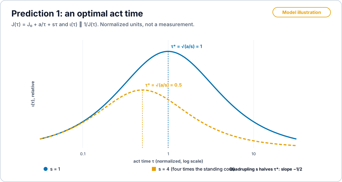
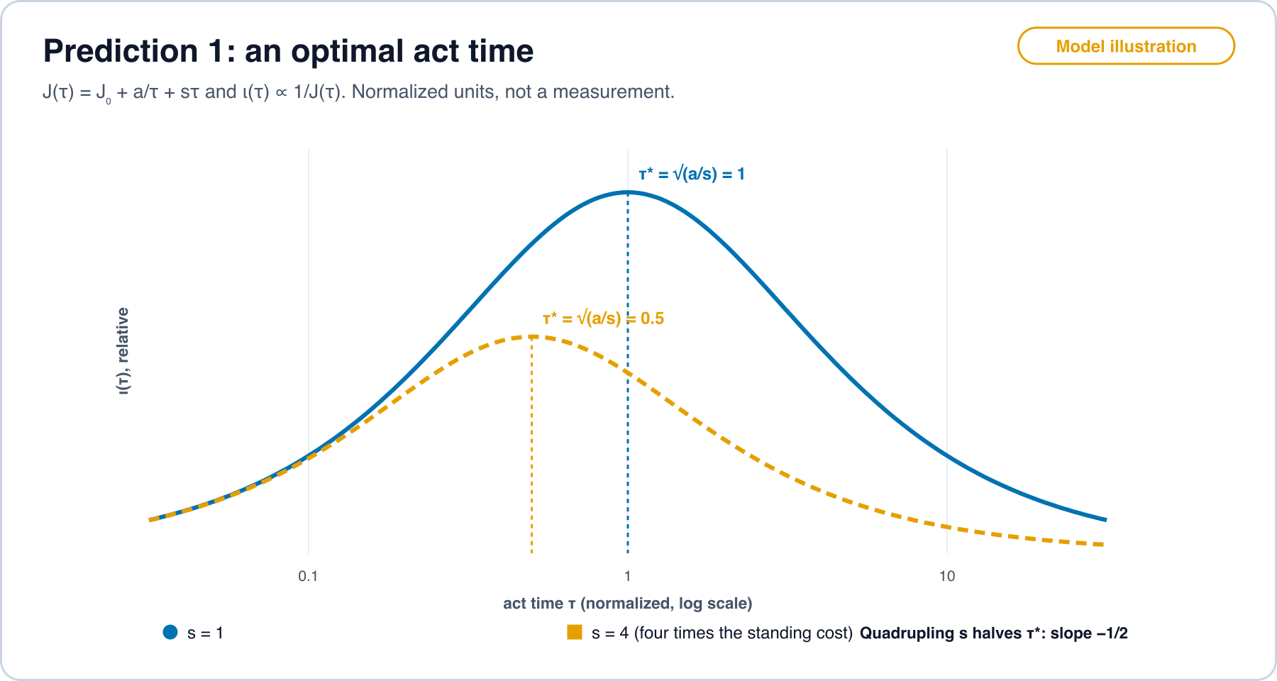
- Optimal act time. Let an acceptor’s measured joules per act follow . Measure and from a sweep of with no goal held, and the standing power from the goal held with no acts. Then the measured peaks at , at the value , with and . The error band is
- Scaling. Across a sweep of the instability rate, falls against with slope .
Falsifier. The measured maximizer of lies outside , or the fitted slope of against over at least one decade of lies outside by more than two standard errors. Either defeats the claim that act joules and standing joules add on one meter, with read as their density. A measured above the ceiling defeats the accounting of that run (F12, Section 8.7).
Figure 2 draws the curve of Prediction 1.
Against the closest work. A finite optimal cycle time is not new by itself. Paneru and colleagues measured a power-optimal cycle time in a Brownian information engine [330]. Panizon derives optimal measurement schedules as a function of measurement cost [331], and Rolandi and colleagues bound an energy, time and accuracy trade-off in thermodynamic computing [332]. What Prediction 1 adds is the source of the interior optimum, a standing cost of holding a goal against drift, and its scaling: falls as . The slope test is the distinctive falsifier.
What is new. The finite-time Landauer bound prices the memory alone and falls toward as grows [29]. There, the slowest reset is the cheapest. The data-rate theorem prices holding alone, per second (Section 4.1). Neither gives an interior optimum. The definition meters the whole agent, counts confirmed bits only, and reads as a density on the joule axis. Then holding a goal makes slowness expensive, and the best act time is the geometric mean of the jump time and the drift time , up to the factor . The controller’s own costs enter the joules in the same way in the work of Ehrich, Still and Sivak (Section 5.1).
Where to test it. A colloidal feedback trap imposes virtual potentials in software and computes work from trajectories at the scale (Section 3.2). One coordinate runs a one-bit act cycle in a virtual double well with reset time . The other is held at the top of a virtual inverted well of rate . A single-electron box with a charge detector runs the same act cycle with every jump counted, so is measured (Section 3.2). Section 8.8 gives the protocol.
Proposition 8. The gated ranking
Setting. Fix a task , its predicate and its allowed failure rate . For each system , is the joules to correct completion of Section 1, with when no policy of passes the gate. Define when .
Statement.
- is a total preorder on systems: reflexive, transitive and total. The ranking of Section 2.3 is its strict part.
- Every system that passes the gate ranks above every system that fails it.
- Let every reading of a policy’s mean joules carry relative error at most . If , then ranks above under every admissible reading.
- Integrated does not induce this order. There are systems with and .
Proof.
- is the pullback of the total order on by the map . A pullback of a total order is a total preorder. Its strict part is , which is the ranking of Section 2.3.
- Every finite value is below .
- Each policy’s reading lies in , so the minimum of the readings over the feasible policies lies in . Then .
- Let make one attempt per task at 0.1 J that passes with probability 1/2 and never retries. Let make one attempt at 1 J that always passes. Each pass credits bits. Then bits per joule and bits per joule. For any , never meets the gate, so , while J.
Reading. Part 4 is the mechanism of R-F6 in Section 8.11: cheap failures raise integrated and leave unchanged or infinite. That is why is read as a density inside a run and is the ranking across systems. Part 3 settles P6 up to a validated for each meter.
Proposition 9. When cheapest first is optimal
Setting. A task has gears . An attempt with gear costs joules, paid in full, and passes with probability . A policy tries gears in some order, stops at the first pass, and refuses after the last. Two structures are treated. Independent: passes of different gears are independent events. Nested: if passes then every later gear passes, with pass probabilities .
Statement.
- Independent gears. The expected joules of an order are least when gears are tried in decreasing order of . Cheapest first is optimal exactly when the order of rising cost is also an order of falling .
- Nested gears, two of them, with the heavy gear sufficient (). Trying the light gear first lowers the expected joules if and only if .
- Budget. Under a hard budget with , light first closes the task with probability . Heavy alone closes it with probability 1.
Proof.
- The expected joules of an order are . Swap two adjacent gears then that follow a prefix with survival probability . Their contribution changes from to , and nothing else changes. So first is no worse if and only if , that is . Any order not sorted by this ratio has an adjacent pair out of order, and swapping it does not raise the expected joules. Finitely many swaps sort the order. This is the ratio rule of Simon and Kadane for search with all-or-none solutions [318].
- Light first costs , because the heavy gear runs only when the light one fails and then passes. Heavy alone costs . The first is smaller if and only if .
- A failed light attempt leaves , so the heavy gear cannot run.
Reading. The fixed cascade, cheapest sufficient first in a fixed order, is optimal when cheap gears pass often enough to pay for their failures: at each step of a nested cascade, or rising cost matched by falling among independent gears. When the condition fails, going straight to the heavier gear wins, and under a binding budget it can be the only way to close. That is the mechanism of the selector result in Section 8.11. The σ-law selector estimates the ratio with calibrated pass probabilities. It is a value-of-computation rule with joules as the cost, in the sense of Russell and Wefald and of Horvitz (Section 5.1). It stops when the next act no longer pays for its joules. Both rules stop at the floor past which more joules buy no verifiable progress, so both are Mixture of Limits instances. P7 (Section 7.1) lists what remains open: a regret bound when pass probabilities are estimated or sufficiency is not monotone, and the nested case with more than two gears, which is a dynamic program over increasing subsequences of gears.
2.4 Where the studies sit
- Mixture of Limits is the optimum operator. The cheapest sufficient gear is the argmin over joules. It is a philosophy, not one fixed order: spend stops at the plateau, where more is waste.
- The receipt carries , , and for every act.
3. Layer 1. The proposed Universal Law of Agency: a definition plus a gate
The definition has four clauses: prediction fixed before the act, coupling to the world through intervention, consequence borne by the system, and a physical floor in joules with refusal on a receipt.
3.0 Objections to the floor
The floor used here is contested, and the assumptions (R1) to (R4) of Proposition 1 are where the objections are met. Norton argues that Landauer’s principle holds only for protocols with a thermodynamically irreversible step [326]. Maroney and Sagawa separate logical from thermodynamic irreversibility: prices the entropy change of a memory, not a bit as such [327, 328]. López-Suárez, Neri and Gammaitoni operated an irreversible logic gate below [329]. Wolpert and colleagues argue that the costs of real computers are dominated by mismatch, modularity and clocking rather than by erasure [320]. Each objection narrows the claim rather than reverses it. Proposition 1 is stated only for a record that meets (R1) to (R4), a reset to a fixed state with equal-energy states and no shared interaction energy, which is the case in which the bound holds; the floor is a lower bound, and every confirmed act of the runs in Section 8.11 that the meter resolved sits more than 14 orders of magnitude above it. K5 has a similar scope: Jordan shows that the Margolus-Levitin bound does not limit the rate of computation by energy without an assumption on information density [324], so K5 is read as a bound on orthogonal state changes, not on clock speed.
3.1 Proven
Information has a price. Landauer showed that a logically irreversible operation dissipates at least per bit [6]. This is the floor under clause 4. Bennett built a reversible Turing machine and showed that only erasure must cost [35]. The unavoidable cost of agency sits at the reset of the acceptor, not at the thinking. Bennett then resolved Maxwell’s demon by the cost of erasing the demon’s memory [7]. The demon is a minimal agent. Its accounts close only when its memory is reset. That is clause 3 plus clause 4.
Feedback is priced by information. Sagawa and Ueda proved that with feedback, extractable work is bounded by [3]. The value of acting on a measurement is capped by the information the measurement carries. They proved that measurement work plus erasure work is at least [5]. The full cycle of predict, compare and reset is priced in joules. They derived an exact Jarzynski equality under feedback [4] and a fluctuation theorem with information exchange between subsystems [36]. Coupling is a correlation that enters the second law. Hartle, Wolpert, Stier, Kempes and Manzano priced feedback with noisy measurements, limited memory and a limited repertoire of protocols. Against random action as the baseline, the benefit of feedback can exceed the information gained by orders of magnitude [37]. The bits bound the work against free energy. The value against a baseline is read off the meter.
Entropy converts to joules. Esposito and Van den Broeck derived for an isothermal driven system [24]. Every kinematic bound in Layer 2 becomes a joule bound through this identity. Horodecki and Oppenheim proved work costs for single shots at small scale [38]. Agency acts are single shots. The standard reviews state the settled account: information is a thermodynamic resource with a price [39, 40].
Control needs coupling. Conant and Ashby proved that a good regulator must be a model of the system it regulates [41]. A system that regulates well already carries a prediction. Touchette and Lloyd proved that the entropy a controller removes is bounded by its mutual information with the system [32, 33]. Coupling is the currency of control. Closed loop control, acting on a comparison, is what the definition requires. Pearl’s do-calculus gives the intervention operator and the conditions under which its effects are identifiable [1]. Clause 2 is written in this operator. Everitt and colleagues classified how an agent can tamper with its own reward or inputs [2]. Coupling must be to the world, not to the agent’s own sensor. Richens and Everitt proved that any agent that meets a regret bound under a large set of distributional shifts has learned an approximate causal model of the process that generates its data [42]. Richens, Abel, Bellot and Everitt proved that any agent that generalizes to multi-step goal-directed tasks has learned a predictive model of its environment, and that the model can be extracted from the policy [43]. A capable agent carries a prediction. That is clause 1, proven for modern agents.
Information flows inside the agent. Horowitz and Esposito showed that information flow between subsystems enters each subsystem’s second law [44]. Coupling becomes a rate. Ito and Sagawa proved a second law for arbitrary causal networks with transfer entropy [45]. Prediction, act and outcome are nodes on such a network. Hartich, Barato and Seifert linked transfer entropy, learning rate and dissipation [46]. Allahverdyan, Janzing and Mahler bounded the efficiency of information flow between coupled systems [47]. Esposito and Schaller showed that feedback that changes only barriers still enters the entropy balance [48]. A purely informational act is in the joule ledger.
Autonomous demons. Mandal and Jarzynski solved a demon that lifts a mass by writing bits to a tape [49]. It has no outside operator, and memory pays for its work. Boyd, Mandal and Crutchfield bounded the work of such ratchets by the entropy rates of their input and output tapes [50]. They showed that modular designs pay dissipation above Landauer [51]. How an agent is built changes its floor. Wolpert and Kolchinsky computed the extra entropy production a gate pays inside a circuit, set by the circuit’s topology [52]. Wiring is part of the floor.
Prediction quality has a joule price. Kolchinsky and Wolpert proved that a process tuned for one input distribution dissipates extra on any other, by a relative entropy term [53]. Still, Sivak, Bell and Crooks showed that memory that does not predict costs dissipation [54]. Keeping only what predicts is the cheap design. Kolchinsky and Wolpert defined semantic information as information that is causally necessary for a system to keep itself out of equilibrium, with a thermodynamic value [55]. It is the closest existing account with joules. It stops before kinematics and before an intelligence operator. Ortega and Braun derived bounded-rational decisions from a free-energy principle with an information cost [56]. Kolchinsky and Wolpert bounded the heat of universal computation by program complexity [57]. Kolchinsky and Wolpert showed that constraints on the available protocols limit extractable work and the value of information [58]. Manzano and colleagues derived fluctuation relations and second-law-like inequalities for computations that halt at random times [59]. A run that stops when its predicate passes is such a computation.
Coupling and boundary rest on theorems. Ay and Polani defined causal information flow through interventions [8]. Transfer entropy does not measure that flow, shown by example [11]. The Markov blanket condition holds only in a narrow range of parameters, by derivation [15], and its definitions in use differ, by counterexample [16]. Every bipartite stochastic process has a causal blanket, by theorem [22]. Definitions 1 and 2 stand on these results.
3.2 Demonstrated
Landauer’s floor, measured. A colloidal bead in an optical double well approached of mean heat as erasure slowed [60]. A feedback trap measured the same approach with high precision and extra cost at short cycle times [61]. The floor rises when the act is fast. That is a Layer 2 effect seen in a Layer 1 experiment. An adiabatic electronic circuit showed the Landauer cost for irreversible operation and dissipation below for reversible operation [62]. The floor binds the reset, not the logic. Nanomagnetic memory bits showed the floor in memory hardware [63]. Erasure with near-zero work appears when the free-energy accounting is complete [64]. The floor is on total entropy, so the receipt must carry the full account. The entropy that enters the bound was measured to have the Gibbs-Shannon form [65]. A single trapped ion showed the quantum floor [66]. The floor holds on every substrate tested. An underdamped micromechanical oscillator reached the floor at high speed [67]. A quantum dot erased bits at minimal dissipation for a given duration, with protocols designed from thermodynamic length [68].
Feedback agents turn information into work. A colloid on a spiral staircase potential gained free energy above the work done, paid by information, and confirmed the generalized Jarzynski equality [69]. This is the first direct observation of an act whose value is set by a measurement made before it. A single-electron box extracted work near per bit [70] and measured the fluctuation theorem with mutual information [71]. An autonomous on-chip demon cooled a system with information while its own heating was measured [72]. The agent’s cost was measured beside its effect.
Quantum agents obey the same bounds. NMR on molecular spins reduced entropy production by feedback, within the information bound [73], and converted information to energy at the floor [74]. Superconducting circuits tracked a demon’s memory during feedback [75], verified the generalized integral fluctuation theorem [76], and measured information gained and lost during feedback [77]. Coupling decays, so the receipt must record it at the time of the act. Cold atoms in a three-dimensional optical lattice were sorted by measurement [78]. Linpeng and colleagues measured the energetic cost of quantum measurement with quantum, coherent and thermal light in a circuit quantum electrodynamics setup. Single-photon light cost the least energy per unit of information gained [79]. The measurement that writes a record has a measured price.
Classical engines measured the price at full scale. An optical tweezer engine converted information to work at the theoretical limit [80]. A colloidal engine extracted work that depends on temporal correlations in its input [81]. A DNA hairpin under continuous monitoring yielded more than per cycle when many measurements happened per cycle, consistent with the information content [82]. A levitated microparticle with delayed feedback obeyed a generalized second law across two decades of delay, and feedback failed at large delay [83]. A late act is a weaker act. Feedback trap engines maximized power and velocity [84], exploited noisy measurements optimally [85], and harvested a nonequilibrium bath [86]. A quantum dot linked work fluctuations to dissipation during information-to-work conversion [87]. A trapped ion verified fluctuation theorems that include the demon’s own dissipation [88], following theory by Zeng and Wang [89].
Functional-system agents built and run. A simulated nematode with an acceptor of action results learned locomotion and chemotaxis [90]. A physical mobile robot ran the same functional-system controller [91]. Clauses 1 and 3 run in software and on a body. Neither meters joules.
3.3 Positions in the literature
Purposive systems and anticipation. Rosenblueth, Wiener and Bigelow defined purposeful behavior through negative feedback toward a goal [92]. It has no energy term. Anokhin’s functional system has afferent synthesis, decision, an acceptor of action results fixed before the act, action, and comparison [93, 94]. This is clauses 1 and 3 in their first systematic form, built on animal experiments. Sudakov stated the result as the system-forming factor [95]. The prediction clause is the organizing principle. Shvyrkov showed from single-neuron recordings that the goal organizes neural activity [96]. Rosen defined an anticipatory system as one that contains a predictive model of itself and its world and acts on the prediction [97]. None of these sets a joule floor. Sterling defines allostasis as regulation by prediction [98]. Physiology puts the prediction before the act. Virgo, Biehl and McGregor gave conditions under which a system’s states can be read as beliefs updated by Bayes’ theorem [99]. Biehl and Virgo call a system an agent when it can be read as solving a POMDP (partially observable Markov decision process) [100]. Both are formal definitions. Clause 1 asks for less and fixes more: one template, fixed at , hashed on the receipt.
Autonomy and organization. Maturana and Varela defined the living by self-production [101]. Kauffman put a thermodynamic work cycle inside the definition of an autonomous agent [102]. It has no prediction clause. Di Paolo made adaptivity, the regulation of one’s own viability, a condition for sense-making [103]. That is clause 3. Barandiaran and Moreno proposed a minimal criterion for cognitive organization and grounded adaptive regulation in metabolism [104, 105]. Barandiaran, Di Paolo and Rohde defined agency by individuality, interactional asymmetry and normativity [106]. Ruiz-Mirazo, Moreno and Mossio framed autonomy as a self-maintaining metabolic organization [107, 108]. Montévil and Mossio described organisms as closures of constraints on thermodynamic flows [109]. It is the closest of this school to joules. Aguilera and Barandiaran built a minimal model of autonomous agency in stochastic thermodynamics [110]. The autonomy tradition is moving toward the joule. Barandiaran and Almendros applied individuality, normativity and interactional asymmetry to large language models. A model fails the first two and partly fails the third [111]. The definition applies its gate per act: a model call is an act when its receipt carries , and . Levin’s TAME (Technological Approach to Mind Everywhere) treats agency as graded and testable by experiment at every scale [112]. The definition keeps the gate binary per act and puts the grading in .
Free energy and the physics of agency. Friston proposes that agents minimize variational free energy [113, 114]. That free energy is informational, not joules, and every bounded system qualifies, so it sets no floor. Rovelli explains agency through the entropy gradient [115]. Agency is thermodynamic at root. Jaeger argues that agency requires self-manufacture and that current artificial intelligence lacks it [116]. That is a demand for a gate before any intelligence claim. Azadi ties agency to computational irreducibility [117]. Wissner-Gross and Freer propose a force toward future path diversity [118]. Its causal temperature is not a bath temperature, so its units are not joules. Kappen’s comment critiques it [119]. Fields, Goldstein and Sandved-Smith separate thermodynamic free energy, in joules, from variational free energy in active inference agents, and relate the two [120]. Only the joule quantity enters K1. Bruineberg and colleagues separate the Markov blanket as a tool of inference from the blanket as a physical boundary [17]. Definition 2 takes the boundary from the definition. Bartlett and colleagues make goal-directed information processing, measured by semantic information, the distinctive feature of living systems [121]. That is clauses 2 and 3 as a criterion for life.
4. Layer 2. The kinematic bounds of agency
Once an act is eligible, physics bounds how fast agency moves per second and per joule, and what precision and speed cost. The bounds come in four families: speed limits, the TUR, finite-time costs and rate ceilings.
4.1 Proven
Speed limits. Shiraishi, Funo and Saito proved the classical speed limit in Section 2.2 [23]. Moving the agent’s state distribution a distance in time costs entropy, and so joules. The bound extends to open quantum systems [122] and to strong coupling with general environments [123]. Vo, Van Vu and Hasegawa derived the speed limit and the TUR from one inequality [124]. Falasco and Esposito bounded the time to complete a transition by the dissipation spent [125]. Ito bounded the information-geometric speed of a distribution by entropy production [126]. Ito and Dechant bounded the rate of change of any observable by Fisher information and dissipation [127]. Nakazato and Ito bounded entropy production by the Wasserstein distance traveled [128]. Dechant, Sasa and Ito split entropy production into the part that moves the system and the part that keeps it running [129]. Van Vu and Saito unified the TUR, minimum dissipation and speed limits through optimal transport [130]. Nagayama, Yoshimura and Ito derived a family of speed limits indexed by generalized means of activity [131]. Yoshimura and Ito proved the TUR and the speed limit in deterministic chemical reaction networks [132]. Aurell, Mejía-Monasterio and Muratore-Ginanneschi solved minimal finite-time dissipation as an optimal transport problem [133]. The kinematic bounds form one family. The cheapest way to move an agent’s state is a transport map. Hasegawa derived the speed limit, the TUR and the Heisenberg principle from one bulk-boundary correspondence [134]. Van Vu and Hasegawa bounded irreversible entropy production by a modified Wasserstein distance in classical and quantum Markov systems [135]. Delvenne and Falasco bounded entropy production by the statistics of kinetic observables [136].
Precision costs dissipation. Barato and Seifert stated the TUR, [25]. A reliable agent pays for its reliability. From at , precision of 1% costs at least 20,000 [137]. Gingrich, Horowitz, Perunov and England proved the TUR for all steady-state currents [26]. Horowitz and Gingrich proved it for finite observation times [138], which is what agents have. Further results bound the full distribution of fluctuations [139], cover discrete time steps [140], extend the TUR wherever a fluctuation theorem holds [141], and cover Langevin dynamics, underdamped motion and velocity feedback [142, 143, 144]. Correlations between currents tighten the bounds [145]. Potts and Samuelsson showed that any fluctuation relation implies a TUR, including with measurement and feedback [28]. This is the precision bound for agents. A review states the field [146]. Barato and Seifert priced the precision of a clock [147]. Salazar bounded entropy production by information from the detailed fluctuation theorem [148]. Landi and Paternostro reviewed entropy production from classical to quantum [149]. Feedback forms now cover the cases agents meet. Van Vu and Hasegawa bounded fluctuations under arbitrary control protocols by entropy production and a kinetic term [150]. Tanogami, Van Vu and Saito bounded the current of a subsystem by its own entropy production and the information flow between it and its partner [151]. Kumasaki, Tojo, Sagawa and Funo derived a TUR for feedback cooling [152]. Honma and Van Vu derived a finite-time TUR for open quantum systems under continuous monitoring and Markovian feedback, with quantum mutual information beside entropy production [153]. For counting observables, Garrahan bounded fluctuations by dynamical activity and gave the matching bounds for first-passage times [34]. Gingrich and Horowitz derived the conjugate relation for the first passage time to accumulate a net current [154]. Proposition 3 applies these results to confirmed agency.
Finite-time costs. Schmiedl and Seifert found optimal finite-time protocols, with jumps at the ends [155]. The optimal act at finite speed is not the slow act. Sivak and Crooks bounded excess work by the squared thermodynamic length over the duration [30]. Proesmans, Ehrich and Bechhoefer found the minimal cost of erasing a bit in time [29, 156]. The Layer 1 floor becomes a Layer 2 curve. Zhen and colleagues stated a universal finite-time bound on reset energy [157]. Speed and efficiency trade against each other by theorem: efficiency at maximum power [158, 159], finite power forbidding Carnot efficiency [160], a three-way trade among power, efficiency and constancy [161], and a universal constraint for low-dissipation engines [162]. Tsirlin and colleagues found minimal dissipation at a fixed rate [163]. Lee, Lee, Kwon and Park tightened the speed limit for highly irreversible processes and obtained a tight finite-time Landauer bound [164]. Van Vu and Saito derived the finite-time quantum Landauer principle and the role of coherence in it [165]. Rolandi and Perarnau-Llobet derived the finite-time Landauer principle beyond weak coupling [166]. Kamijima, Funo and Sagawa derived the finite-time trade-offs between measurement and feedback [167]. Tkachenko showed for physical neural networks that quasi-static inference needs no work, while finite-speed inference costs at least a transport distance (preprint) [168]. Inference has no floor that survives slow operation. The reset does. Proposition 1 prices it.
Holding a goal. Tatikonda and Mitter [169] and Nair and Evans [170] proved the data-rate theorem: holding an unstable linear system needs a channel rate above the sum of the base-2 logarithms of its unstable eigenvalue magnitudes. Nair, Fagnani, Zampieri and Evans reviewed the field [171]. Sandberg, Delvenne, Newton and Mitter found the maximum work a continuously measuring demon extracts in finite time, and showed that any implementation needs an external power source [172]. Horowitz and Sandberg showed that the information terms in second-law inequalities form a hierarchy, each the minimum cost of acquiring that information by a distinct measurement [173]. Proposition 2 turns the bit count into a joule floor per step. It is a joule-priced corollary of the data-rate theorem, not a new law.
Quantum feedback and measurement. The feedback second law holds for quantum systems [3]. Jacobs extended it to weak measurements [174]. Funo, Watanabe and Ueda derived integral fluctuation theorems under quantum measurement and feedback [175]. Guryanova, Friis and Huber proved that ideal projective measurements need infinite resources, and gave the energy cost of a pointer that reproduces the system’s statistics [176]. Danageozian, Wilde and Buscemi bounded the measurement heat of error identification by the Groenewold information gain [177]. These price the measurement that writes a record. Proposition 4 keeps the floor of the record itself.
Groups. Wolpert derived a strictly nonzero lower bound on the minimal entropy production rate of interacting subsystems from the constraints on which subsystems each one depends on [178]. Tasnim and Wolpert extended the theory to subsystems that change state together [179]. Wolpert related the entropy production of a whole Bayes net to the precision of currents in its parts [180]. Rolandi, Abiuso and Perarnau-Llobet showed that collective protocols can make dissipated work grow sublinearly with the number of members [181]. Fujimoto and Ito found by a game-theoretic method that the partial entropy productions of interacting subsystems trade against each other, and that the total is least when the subsystems share the penalty equally [182]. Proposition 7 composes these joules with the group’s coupled bits.
Rate ceilings. Margolus and Levitin bounded orthogonal transitions per second by energy [31]. Lloyd applied the limit to a whole computer [183]. Deffner and Campbell reviewed the family of quantum speed limits [184].
Living sensors. Energy dissipation, adaptation speed and accuracy are bound together in bacterial chemotaxis [185]. Learning about the environment requires energy [186], and inference accuracy is tied to dissipation [187]. Sensing precision is limited by receptors, time and energy, with an optimal allocation among them [188]. No resource can be skipped. That fits Mixture of Limits. Erasure inside adaptation has a cost [189]. Information acquired per energy dissipated is the nearest existing quantity to in living sensors [190, 191]. Copying information costs energy [192]. Writing the receipt has a price. Accurate and synchronized biochemical clocks cost free energy [193, 194], and so does reducing noise at high sensitivity [195]. Holding a system away from equilibrium has a minimum power [196]. That is the standing cost of an agent ready to act. Bryant and Machta bounded the energy of sending a bit through a cell’s physical channels, in per bit, as a function of size, distance and latency, and found it many orders of magnitude above unity [197]. Tjalma and colleagues showed that the bits of the past that best predict the future are prohibitively costly for cellular networks [198].
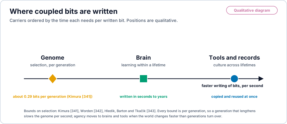
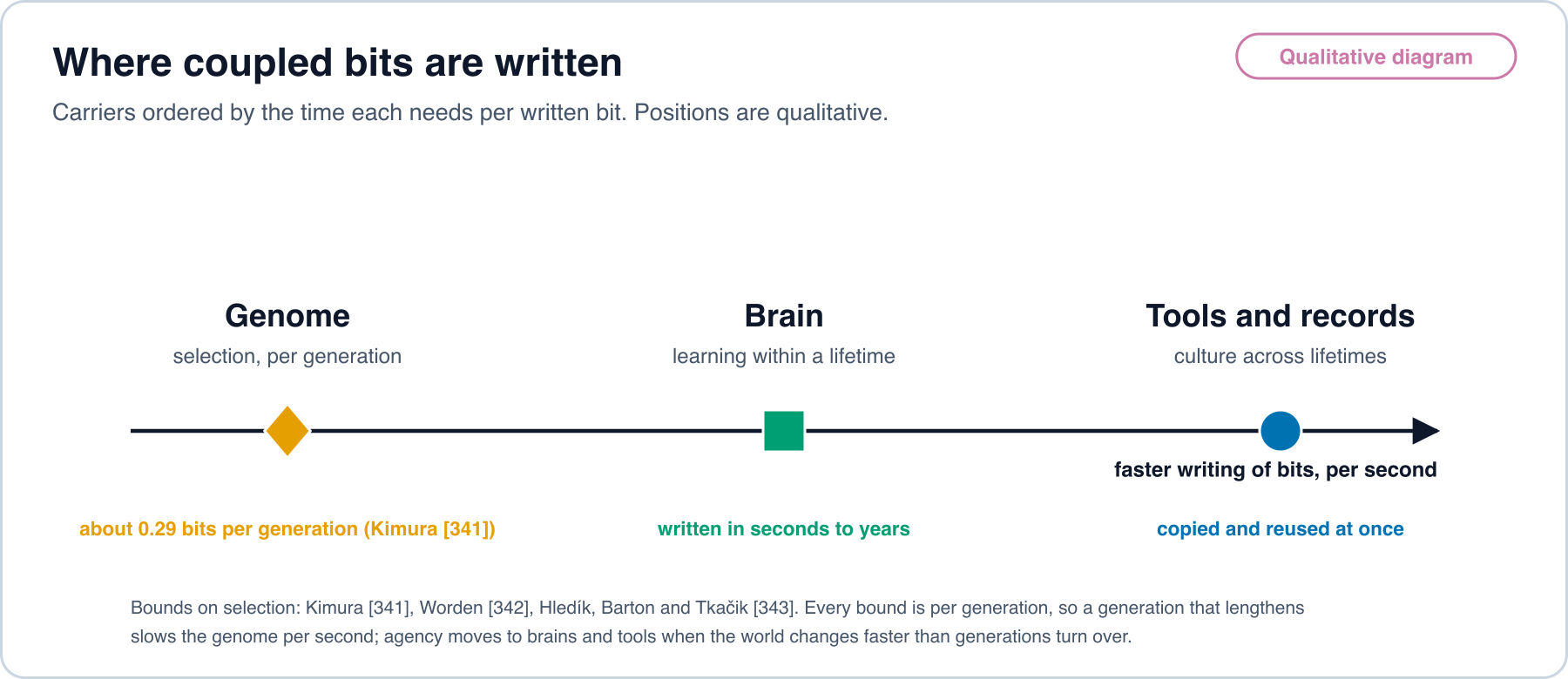
Information gained by selection. Selection also writes bits, and its rate is bounded. Kimura measured the information that natural selection accumulates in a genome by the substitutional load and, with the load values he took as representative, estimated about 0.29 bits per generation [341]. Worden bounded the rate at which selection can add information to a genome in terms of the selection applied per generation [342]. Hledík, Barton and Tkačik showed that, in stochastic populations, the rate is bounded by the population size times the cost of selection, across Wright-Fisher, Moran and diffusion models [343]. Every such bound is a rate per generation. A generation lengthens as an organism grows, so a carrier that learns only through selection gains coupled bits ever more slowly per second. Nervous systems write bits within a lifetime, and cultural records write them across lifetimes. The kinematics of Section 2.2 apply to each carrier. What changes from one carrier to the next is the time per written bit, which is the reason agency moves from genomes to brains to tools when the world changes faster than generations turn over.
Figure 3 orders the three carriers.
Information rates without joules. Schreiber defined transfer entropy, directed information flow per step [199]. It is per time, not per joule, and it has no eligibility gate. Tishby and Polani charged information per step in a Bellman recursion [200]. Landauer converts those bits to joules. Stratonovich bounded the maximal gain from a given amount of information [201]. That is a ceiling on value per coupled bit.
4.2 Demonstrated
The TUR tested. A two-qubit NMR experiment obeyed generalized TURs and violated the specialized TUR where theory predicts [202]. An optical tweezer information engine violated the original TUR near maximal efficiency and obeyed generalized bounds with mutual information [27]. Agents need the feedback form. A quantum dot Szilard engine confirmed it independently [203]. Atomic-scale conductors examined the TUR with measured current noise, the physics of every chip [204]. Molecular motors were scored by precision per unit dissipation [205]. Observed current fluctuations bound dissipation from below [206]. A receipt of fluctuations is a lower-bound meter for joules.
Speed limits and finite-time costs tested. Single atoms in an optical lattice showed the Mandelstam-Tamm and Margolus-Levitin bounds and the crossover between them [207]. The rate ceiling is measured. A trapped colloid measured time and entropy trade-offs for fast thermal transitions [208]. Brownian particles driven by optimal transport protocols saturated the minimal finite-time dissipation bound [209]. The kinematic optimum is reachable. A feedback trap measured a two-force Brownian machine against linear response bounds [210]. A photonic experiment tested geometric bounds on entropy production [211]. Dago and Bellon measured erasure in a double-well memory at high speed and traced the overhead above Landauer’s bound to its sources [212].
Living sensors measured. Mattingly, Kamino, Machta and Emonet measured the rate at which E. coli acquires information during chemotaxis, and showed that the cells climb gradients close to the limit that rate sets [213]. Information limits behavior, measured.
Heat engines at finite speed. A single colloid ran a micrometer Stirling engine [214]. A trapped bead ran a Brownian Carnot cycle with efficiency at maximum power measured [215]. The energy cost of choosing one of two options was measured [216]. That is the smallest act. A colloidal engine ran on an active bacterial bath [217], and engineered noise gave near-Carnot efficiency at finite power by shortening relaxation [218]. Engineering activity moves the bound. An information engine flipped from refrigerator to heater with noise [219]. The receipt must record the regime, not only means.
Empowerment in simulation. Klyubin, Polani and Nehaniv defined empowerment, the channel capacity from actions to future sensors [9]. It was computed for continuous control [220] and reviewed [221]. It measures how much an agent can move the world, in bits. It is not a rate per joule.
4.3 Positions in the literature
Kinematics is mostly theorem and experiment. The opinions here concern which variable is right. Seifert holds that inference from fluctuations is the route to hidden costs [137]. Rovelli and Wissner-Gross and Freer both propose entropic kinematics [115, 118]. Kolchinsky shows that dissipation alone does not bound how fast replicators grow or decay [222]. Rates are bounded by dissipation together with activity. That is the form of the speed limit, where sits beside . Adlam, McQueen and Waegell argue that a purely quantum system cannot be an agent, because building a world model and deliberating need copying, which the no-cloning theorem forbids (preprint) [223]. Clause 3 already asks for a classical record of .
5. Layer 3. Intelligence as the calculus of agency
Intelligence is the derivative of gated agency in joules, read off a completed run. This layer needs three things from the literature: theory that ties learning and decision to joules, measurement of joules per unit of useful work, and positions on what intelligence is.
5.1 Proven
Learning and prediction priced in joules. Goldt and Seifert bounded the information a learning network acquires by the entropy it produces [224]. Learning efficiency is at most one. This is for the learning part of an act, with a ceiling. Still showed that optimal memory keeps only predictive information [225]. The marginal joule spent on memory must buy prediction. Boyd, Crutchfield and Gu proved that the agent that extracts the most work from data has the maximum-likelihood model of that data [226]. Better models yield more work per joule. Boyd, Crutchfield, Gu and Binder stated overfitting and generalization as energetics [227]. Generalization appears as joules. Ehrich, Still and Sivak priced the controller itself, beyond the information it uses [228]. So must be metered at the wall of the whole system. Ehrich and Sivak gave the ledger of energy and information flows in autonomous machines [229]. Wolpert reviewed computation costs beyond Landauer [230]. Wolpert and colleagues set out the open problems for the energy costs of computation in stochastic thermodynamics [320]. Levy and Baxter showed that neural codes that maximize bits per unit energy differ from codes that maximize bits [231]. The right objective for a brain is information per joule. Balasubramanian, Kimber and Berry set the objective for an exploratory regime as transmission rate per unit power [232]. That is bits per joule. Goldt and Seifert bounded the information a network learns about a rule by the thermodynamic cost of learning, for batch and online learning [233]. Fiderer, Barth, Smith and Briegel defined the work capacity of an environment channel, the maximum rate at which any agent can expect to extract work in a percept-action loop. Work-efficient agents balance prediction against forgetting (preprint) [234]. Elliott, Gu, Garner and Thompson showed that quantum adaptive agents can need far less memory than memory-minimal classical agents [235]. Less memory to reset is a lower floor to pay.
Decisions and bounded optimality. Russell and Subramanian defined bounded optimality: the best program for a given machine and environment [236]. Here the resource is joules, and the optimum is subject to . Russell and Wefald priced each computation by its expected effect on the decision, net of its cost, and stopped deliberation when no computation had positive net value [316]. Horvitz framed the same trade for reasoning under resource constraints [317]. The σ-law selector is that rule with the cost in metered joules. Proposition 9 gives its exact form for a cascade. Genewein and colleagues derived abstraction and hierarchy from utility minus information cost [237]. Mixture of Limits gears are such a hierarchy. Legg and Hutter defined intelligence as complexity-weighted expected reward over all computable environments [238]. It is an integral, but over reward, without energy, and uncomputable. The derivative in joules replaces reward with confirmed coupled bits and the measure with metered joules. Takahashi and Hayashi give the closest existing calculus in joules [239]. They define two ratios under explicit accounting conventions. Thermodynamic epiplexity per joule is : new bits about an environment variable retained in the agent’s state, per joule consumed inside a stated boundary. Empowerment per joule is the capacity of the channel from acts to observations per unit expected energetic cost, the capacity-per-unit-cost of Verdú. They prove a closed-cycle Landauer benchmark by joining a thermodynamic learning inequality with data processing, and they show by a reversible copying construction that, with an open boundary and fresh memory brought in free, information gain and in-boundary dissipation decouple. They close with a reporting checklist: boundary, energy balance, baseline, coarse-graining, horizon and reset, throughput, estimator. This track takes four things from that work. Their closed-cycle benchmark is K1 for learning. Their decoupling construction is the reason for act-closed metering in Definition 2 (Lemma 1). Their checklist is adopted in Section 8.12. Their advice to report bits per joule beside bits per second is the variable Prediction 1 optimizes. The definition differs from their metrics in four exact ways. Empowerment per joule is a capacity, a supremum over act distributions; the definition credits the realized flow of the policy that ran (Definition 1), with capacity as its bound. Their numbers are benchmark-relative efficiency reports, by their own statement; this track ranks systems by behind a correctness gate (Proposition 8). They have no prediction fixed before the act, no consequence clause and no refusal; the definition requires all three before any bit counts. They give no kinematics of time; Prediction 1 derives an optimal act time and a ceiling from the same joule accounting. Ortega, Braun, Dyer, Kim and Tishby set out information-theoretic bounded rationality [240]. Zénon, Solopchuk and Pezzulo cast the cost of cognition as information [241]. Sims applied rate-distortion theory to perception [242]. Their currency is bits. Landauer converts bits to joules at the reset.
5.2 Demonstrated
Brains. Laughlin, de Ruyter van Steveninck and Anderson measured the energy cost per bit in blowfly photoreceptors and interneurons [243]. Higher information rates cost more per bit. That is a measured in a living agent and a measured diminishing return, in sensing. Attwell and Laughlin built the energy budget of grey matter by process [244]. Lennie showed that energy limits how many cortical neurons can be active at once [245]. Energy is the constraint, and the rest adapts. Energy per action potential differs widely across neuron types [246]. Same function, different joules. Neural design follows energy efficiency [247]. Levy and Calvert audited the human cortex. Communication costs 35 times as much as computation, and a neuron’s computation sits a factor of from the best possible bits per joule [248]. That is a distance to the floor. Harris and colleagues found that a visual pathway synapse is sized to maximize information per unit energy, not information [249]. The objective is bits per joule, measured at one synapse. Padamsey, Katsanevaki, Dupuy and Rochefort found that food restriction cut synaptic ATP (adenosine triphosphate) use in mouse visual cortex by 29% and broadened orientation tuning by 32% [250]. Fewer joules bought less precision. Plaçais and Preat showed that starved flies switch off costly aversive long-term memory, and forcing it back reduced survival [251]. Plaçais and colleagues found that raised energy flux in the mushroom body triggers long-term memory [252]. Mery and Kawecki found that forming long-term memory lowered flies’ resistance to desiccation [253]. Learning has a measured metabolic price. Hechler, de Lange and Riedl measured lower cortical oxygen use during confident prediction, by up to 12% (preprint) [254]. Prediction first can save joules. Malkin and colleagues gave synapses an energy cost for reliability in trained networks and found signatures of Bayesian inference in the optimum [255]. Li and van Rossum showed that naive synaptic plasticity costs extreme energy and that caching changes before consolidation saves it [256]. Lynn and colleagues inferred broken detailed balance in the human brain from neuroimaging, rising with physical and cognitive exertion [257]. That entropy production is coarse-grained and informational. It is not a joule meter.
Machines. Memory access costs far more energy than arithmetic [258]. Parameter count matters only through the joules it makes you move. Intelligence per watt measures task accuracy per unit power on local accelerators [259]. Its numerator is benchmark accuracy, not gated agency. MLPerf Power standardizes power measurement from microwatts to megawatts, with each result gated by an accuracy target [260]. That gate is the form of . FrugalGPT cascades language models and stops when a scorer accepts the answer [321]. RouteLLM learns to send each query to a strong or a weak model under a cost target [322]. Their cost is dollars per query and their gate is a quality threshold. Read with metered joules and as the gate, both are cascades in the sense of Proposition 9. ML.ENERGY measures inference energy automatically [261]. TokenPowerBench benchmarks the power of large language model (LLM) inference [262]. Jin, Wei and Brooks analyze the energy of test-time compute [263]. General-purpose models cost much more energy per task than task-specific ones [264]. The cheapest sufficient model wins in joules. That is Mixture of Limits, measured. Samsi and colleagues measured the energy of large language model inference on GPUs (graphics processing units) [265]. Dillavou and colleagues demonstrated decentralized learning in a physical circuit, with no processor [266]. Stern and colleagues trained self-learning circuits for power-efficient solutions and measured the trade between power and error [267]. Saggio and colleagues demonstrated a quantum speed-up for learning agents in a photonic experiment [268]. Fewer interactions to learn is fewer acts to close.
A kernel-reported acceptor. Section 8.11 reports a preregistered run of an acceptor agent on a laptop, with prediction first, comparison, refusal and binding joule budgets. Falsifiers were fixed before the run, and several fired: R-F1 (the selectors’ joules on shared tasks are not distinguishable), R-F2 (36 of 5,400 episodes overspent: 9 for the σ-law arm and 7 for the fixed cascade at , and 20 for the goal-blind baseline at ), R-F3, R-F5 and R-F6 (Section 8.11). was read off 4,940 receipts. The median confirmed act gave bits per reported joule, about times the joules per bit of the floor. Under a binding budget the σ-law selector closed more tasks than the fixed cascade, one Mixture of Limits instance. That comparison was chosen after the run, so it is exploratory, and joules per closed task were equal. The preregistered second run and a second machine repeated the gain at the loosest budget only (Section 8.11.2). Integrated ranked a goal-blind agent first on a loose budget, while ranked it last.
Groups simulated. Crosato and colleagues computed the thermodynamic quantities of simulated collective motion across its critical point [269]. Chen and Prokopenko compared thermodynamic efficiency with purely informational utilities as explanations of collective behavior near criticality [270]. in Proposition 7 is the gated, metered form of such a ratio.
Meters. RAPL (Running Average Power Limit) is the set of on-die energy counters in Intel and AMD processors. Its readings were validated against external measurement [271]. DRAM (dynamic random-access memory) readings were validated separately [272]. Meter quality depends on the processor generation [273]. Apple’s powermetrics manual states that its average power values “are estimated and may be inaccurate” and should not be used to compare devices [274]. On Apple silicon, powermetrics readings are reported values. Measured joules for that machine come from an external wall meter.
Compression scored. The Hutter Prize scores lossless compression of the first gigabyte of an English Wikipedia dump, with a prize fund of 500,000 euros and limits on runtime and memory [275]. It bounds time and memory, never joules. A joule cap would make it a calculus-of-agency benchmark for one task class.
Estimates. These sources are valuable, and their joule figures are modeled, extrapolated or computed. They sit beside measured joules, never in their place. Estimates are never measured_j. Strubell, Ganesh and McCallum sampled power for short runs and extrapolated to full training of natural language processing models [276]. Patterson and colleagues computed training energy from reported hardware, runtime and data-center data [277]. Lacoste and colleagues built a calculator from hardware type, runtime and region [278]. The BLOOM footprint mixes metered and modeled inputs [279]. Carbontracker reads on-device counters and predicts full-run totals [280]. Its predictions are estimates. Elsworth and colleagues report a median of 0.24 Wh per Gemini Apps text prompt, counting accelerators, hosts, idle capacity and data-center overhead [281]. It is an operator-reported figure, filed as reported_j.
5.3 Positions in the literature
Each position is placed against the definition: intelligence is the derivative of gated agency in joules, read off a completed run.
- Schmidhuber treats intrinsic reward as compression progress, a first derivative of how well an agent compresses its history [282]. It is the closest precedent for intelligence as a derivative read from a run. Its variable is compression, not joules.
- Krakauer, Mitchell and Krakauer define intelligence as an emergent property expressed in ever cheaper and faster uses of emergent capabilities to solve problems, summarized as “less is more” [339]. They conclude that large language models show emergent capability at most, not emergent intelligence. Their definition is the closest in words to . It names energy as the denominator and does not meter it. The calculus supplies the meter, the gate that separates capability from intelligence (Section 1), and the derivative read off the run.
- Chollet defines intelligence as skill-acquisition efficiency over priors and experience, with the ARC (Abstraction and Reasoning Corpus) benchmark [283]. It is a ratio. Its denominator is information and data, not joules. The ARC Prize leaderboard plots cost per task against score as a measure of efficiency [284]. The cost is in dollars. A joule meter turns it into .
- Hernández-Orallo builds universal psychometrics across species and machines [285]. It evaluates by tasks. This track evaluates by joules to close tasks. Hernández-Orallo and Dowe’s anytime test adapts to the time available [286]. The calculus adapts to the joules available.
- Gershman, Horvitz and Tenenbaum define intelligence as expected utility net of computation cost [287]. This track makes the cost joules.
- Lieder and Griffiths treat cognition as optimal use of limited resources [288]. It is close to Mixture of Limits. The resource is left abstract.
- Balasubramanian reads the brain’s design through its energy limits [289].
- Silver, Singh, Precup and Sutton hold that reward is enough [290]. Reward is chosen by a designer. Joules are read off a meter. Vamplew and colleagues reply that scalar reward cannot express multi-objective goals [291]. This track keeps one variable, joules, and moves multiplicity into the gate .
- Hafez and colleagues define agency and intelligence together [292]. It is not joule-native.
- Karagoz makes energy self-sustainment the objective [293]. It has no prediction gate, no kinematics and no joule ranking across systems.
- Chaisson proposes energy rate density, power per unit mass, as a complexity metric across cosmic evolution [294]. It is a rate in watts per kilogram. The calculus divides confirmed bits by joules.
The scope of follows from its numerator. counts confirmed coupling to the world, so measures how cheaply an agent changes the world as it predicted. It does not measure understanding. Krakauer, Mitchell and Krakauer tie intelligence to compact, communicable representations [339]. A compact representation enters the calculus through its effect: an agent that holds one closes later tasks in fewer joules. Understanding that never changes an act is outside what reads.
5.4 Where the calculus stands
- Proven: learning, memory, prediction and control each have a joule price with a ceiling.
- Demonstrated: joules per bit are measured in brains. Joules per task are measured in machines. Meters can be validated.
- Proven here: is a bounded density on the joule axis under joule-proportional crediting (Proposition 5). Sampled converges to it (Proposition 6). Groups compose by Proposition 7. Holding a goal sets an optimal act time and a ceiling on (Prediction 1).
- Demonstrated here: and read off the receipts of a kernel-reported acceptor, with falsifiers fixed in advance (Section 8.11). ranks agents. Integrated does not.
- Added by this track: intelligence read as off a gated, completed run, with as the ranking. Takahashi and Hayashi come closest, with bits-per-joule ratios under explicit accounting [239]. This track adds the eligibility gate, the realized flow in place of capacity, the gated ranking and its proof (Proposition 8), and the optimal act time (Prediction 1).
6. Global findings, by method
The search ran in Russian, Chinese, Japanese, German, French, Spanish, Portuguese, Korean, Italian, Polish, Hindi and Arabic, with English follow-ups. A second pass searched Japanese, Chinese, Russian, German, French, Spanish and Korean again and added Persian, Turkish and Hebrew. Its results are folded into Sections 2 to 5 and 8 by what they prove, measure or define. Results are organized by method and class of result. Language is metadata only. No entry is ranked by where it came from.
6.1 Theorems and reviews: information has a thermodynamic price
- Poplavskii gave an early systematic treatment of the energy cost of acquiring and processing information [295]. Written in Russian, with an English translation. Layer: definition.
- Stratonovich proved value-of-information theorems [201]. English edition of a Russian monograph. Layer: kinematics.
- Ito and Sagawa applied information thermodynamics on networks to E. coli chemotaxis. Transfer entropy bounds robustness, and information-thermodynamic efficiency is high where ordinary thermodynamic efficiency is low [296]. Written in Japanese. Layers: definition and kinematics.
- Sun and Quan reviewed Maxwell’s demon and the physical floor on dissipation in information processing [297]. Written in Chinese. Layer: definition.
- Quan, Dong and Sun reviewed mesoscopic thermodynamics: the demon is consistent with the second law once erasure is counted, and power-efficiency constraints were tested [298]. Written in Chinese with an English abstract. Layers: definition and kinematics.
- Parrondo’s encyclopedic review gives the current account of information as a thermodynamic resource [299]. Layer: definition.
- Strasberg’s doctoral thesis tests common assumptions in information thermodynamics with physical models [300]. Written in English with a German abstract. Layer: definition.
- Further theorems surfaced through searches in Japanese, Russian, Chinese, Korean, Portuguese, Italian and Polish: speed limits and TURs in chemical networks [127, 131, 132], finite-time thermodynamics [159, 162, 163], Langevin TURs [143, 144], information bounds on entropy production [148, 149], and single-shot work costs [38].
6.2 Experiments: the price measured
- Dago’s doctoral thesis reports 1-bit erasure and writing near the minimal energy at high speed on an underdamped micro-cantilever [301]. Written in French. Layer: the definition’s joule floor reached at kinematic speed.
- Lagoin’s doctoral thesis builds macroscopic Maxwell’s demons, including a Szilard engine, from a vane in a granular gas [302]. Written in French. Layer: definition. The demon’s accounting holds outside the microscopic regime.
- Ciampini and colleagues used extractable work to witness quantum correlations in a photonic experiment [303]. Layer: definition.
- Experiments surfaced through searches in Korean, Portuguese, Hindi, Italian, Spanish, Chinese and Japanese: information engines [27, 80], NMR demons [73, 74], the TUR on qubits [202], active-bath engines [217, 218], geometric bounds [211], symmetry breaking and Carnot cycles [215, 216], trapped-ion demons [66, 88], and feedback conversion and optimal transport [69, 76, 209].
6.3 Theory of functional systems: prediction before the act
The Anokhin school states clauses 1 and 3 in physiological terms. A result template, the acceptor of action results, is formed before the act, compared after it, and the comparison reorganizes behavior. These works were found through Russian-language searches.
- Anokhin’s functional system [93, 94].
- Sudakov on the result as the system-forming factor and on probabilistic prediction of behavior [95, 304, 305, 306].
- Shvyrkov on goals organizing neuronal activity and on learning as selection of neuronal systems [96, 307].
- K. V. Anokhin on the brain’s cognitive structure as a hypernetwork of functional-system elements [308].
- Saltykov and Grachev on the system-forming factor as anticipation [309].
- Vityaev on purposefulness formalized as rule learning that predicts results [310].
Implemented and run. Cognitive architectures built on functional-system theory form result templates, compare, and learn subgoals, in simulation and on a physical robot [90, 91, 311, 312, 313]. None meters joules. Adding a meter to one of these agents would test the full order of definition, kinematics and calculus on an existing implementation. Differentiable probabilistic logic networks are related calculus tooling, not built on functional systems, with no eligibility gate and no joules [314].
6.4 Autonomy, organization and minimal agency
Found through Spanish, French and German searches. Agency is a self-maintaining organization that regulates its interactions [103, 104, 105, 106, 107, 108]. The organization is a closure of constraints on thermodynamic flows [109]. The autonomy school has stepped into stochastic thermodynamics [110]. Layer: definition, as the organization that must exist before any act counts.
6.5 Measured joules for machine intelligence
Found through Chinese-language searches on inference energy: automated inference energy measurement [261], per-token power benchmarks [262], and the energy of test-time reasoning [263].
6.6 Philosophy of agency
Rovelli’s physics of agency surfaced through German [115]. Jaeger and Azadi complete the set of position papers [116, 117].
6.7 Searches with no primary research
Hindi and Arabic searches returned no primary research in those languages. English follow-ups surfaced further work, listed above by method. Persian, Turkish and Hebrew searches returned theses, reviews and work already cited, with no new primary research.
6.8 Convergence observations: information, energy and prediction
Eleven recent sources relate information, energy and prediction, or the compute spent per generated answer. Four were read in full and are cited for what they state: Takahashi and Hayashi [239], Perrier [344], Xu and Li [345] and Still, Sivak, Bell and Crooks [54]. Seven were read in part and are cited only for the passages named: Wolpert [230], Ortega and Braun [56], Zhang, Zhu, Zhang and Hu [348], Fagan [346], Kumar [347], Kumbong, Khare and colleagues [349] and Zou and colleagues [350]. This section records what each states and what it does not show. It is an observation of overlapping questions, not a comparison of results and not a claim about priority. Section and equation numbers are those of the versions named. Quotations were checked by script against the saved texts. Values marked “recomputed” are this paper’s own arithmetic.
In plain words
- Several authors write the same kind of quantity: information gained or acted on, divided by energy spent (bits per joule), or its inverse (watts per unit of intelligence).
- The firm results are lower bounds on heat. They say how little energy is physically required, not how much any real machine uses.
- No source read here measured energy on real hardware. Where energy figures appear, they are estimated from FLOP counts or from model assumptions.
Units. J/K. At K, J per bit (recomputed), and its inverse is bit/J (recomputed). With , information in nats converts to joules by multiplying by , and in bits by .
Sources read in full
Takahashi and Hayashi, arXiv:2602.05463v2 (20 July 2026) [239]. The version read is the arXiv posting.
- Epiplexity per joule is in bit/J, with (Eqs 3 and 10, Sec 2.2). The energy balance is (Eq 1).
- Empowerment per joule is in bit/J (Eq 18, Sec 3.2), with a cost-constrained curve (Eq 19). Empowerment is a channel capacity from actions to later observations (Eq 17, Sec 3.1).
- The closed-cycle bound is (Eq 15), so when (Eq 16, Corollary 1). Eq 15 follows from Eq 14 by rearrangement (checked). Corollary 1 needs the bipartite-Markov and local-detailed-balance assumptions.
- The authors give a bits-per-joule metric for learning, another for control, and a reporting checklist: boundary, baseline energy, horizon, estimator (Sec 5.1). Their Proposition 1 is a decoupling construction showing the bound fails if the accounting boundary excludes the cost of preparing fresh memory.
- Scope as stated: “the resulting numbers are benchmark-relative rather than universal”. On the ceiling: “Landauer-scale limits are conceptual yardsticks far beyond current hardware.”
- The Sec 5 worked example uses published perplexities, tokens, and energy estimated from FLOPs at an assumed FLOP/J. Recomputed: bit, (410M model) J, marginal efficiency bit/J. The authors write: “This number is convention-dependent, but it exercises the checklist.”
- Not verified here: Lemma 1 restates an inequality from work not read. Eq 17 uses while the Sec 3.2 text refers to . Eq 20 is flagged by the authors: “This is not claimed as a universal identity without assumptions”.
Perrier, arXiv:2504.05328v2 (16 June 2025) [344]. Definitions only are cited.
- Watts per intelligence is (Eq 7, Sec 3.3), where is a task-weighted performance sum (Eq 2) or the Legg and Hutter sum (Eq 1). The assumptions are with and overhead (Eq 5), and with unspecified (Eq 6). Theorem 1 gives (Eq 8).
- The author states the premise openly: “Our work assumes a correlation between irreversible computation to intelligence.” The paper contains no measurement; it says only that “In practice, one might measure the actual hardware usage”.
- Errors found (my reading, not confirmed with the author): (1) Sec 3.1 defines per unit time, but Eqs 3 and 5 use over , which needs as a total, and then falls to zero as grows. (2) is free, so Theorem 1 gives no numerical floor. (3) The Theorem 2 proof yields a bound of the form , which is negative for , yet the text treats as positive. (4) Combining with gives , while Eq 14 has no , no and the opposite dependence on . (5) can be negative, and the direction of the Landauer attachment in Eq 13 is not argued; Theorem 3 inherits this. (6) The hardware ordering is asserted with no values.
Xu and Li, arXiv:2511.19156v4 (30 December 2025) [345]. Read in full for the saved text; figures were read by caption and printed values only. Definitions only are cited.
- Derivation depth (Eq 10) and derivation entropy with nats in a stated classical regime (Eq 14, Assumption 3). Claimed bounds: (Proposition 4, Eqs 98 and 99) and (Proposition 5, Eq 100). A break-even query frequency between recomputing and storing is given in abstract cost units (Theorem 5, Eq 32).
- The authors call their cost an “information-theoretic proxy for energy consumption”. The numerical validation (Sec VI) uses a synthetic 100K-atom knowledge base and the paper’s own abstract costs, so it tests the model against itself. Application figures (1000 kWh, 45 percent reduction) come without a measurement method and are not used here.
- The abstract says “Our findings suggest that the minimization of Derivation Entropy is a governing principle”. The text elsewhere declines to claim a sharp result: “We deliberately refrain from formalizing” the last observation as a phase-transition theorem.
- Errors found (my reading, not confirmed with the authors): (1) Assumption 1 has with an action in J s, while Corollary 1 sets , an energy, and drops . (2) Eq 98 assumes every inference step erases a bit (Assumption 3), and Remark 15 of the same paper concedes reversible computation avoids this cost. (3) In Lemma 2 the contradiction argument negates the bound to and claims this contradicts ; it does not, since . The lower bound is therefore unproved, and Theorems 4 to 6 and Corollary 7 depend on it. (4) Theorem 6 case (b) uses where is needed. (5) The Eq 135 critical storage with recomputes to (log base 2), (ln) or (log base 10), not the printed . The Table II text (tightness 0.50 to 0.93) disagrees with the table (0.50 to 0.81, and 0.89 at high frequency).
Still, Sivak, Bell and Crooks, arXiv:1203.3271v3 (5 October 2012) [54]. The arXiv version was read; the journal version was not.
- With system state and driving signal , and , in nats. Per step, (Eq 14). In total, (Eq 18). The refined Landauer bound is (Eq 21).
- Memory of the signal that does not help predict its next value costs dissipated work, at per nat. The authors’ stated consequence: “any system constructed to keep memory about its environment and to operate with maximal energetic efficiency has to be predictive”.
- This is a lower bound on dissipation for systems that keep memory of a driving signal. It does not show that any real system attains it, and it is not a statement about general agents. There is no experiment and no joule data.
- Checked: footnote 24 is correct; Eq 17 follows from Eqs 11, 14 and 15; Eq 18 follows from Eq 16; Eq 21 follows from Eqs 19 and 20. meV at 300 K (recomputed; the paper gives 25 meV). Not verified: non-negativity of the per-step term for arbitrary signal processes is stated but not proved in the text, and it is not proved here.
Sources read in part
Each entry is limited to the passage stated. No claim is made about the unread parts.
-
Wolpert, arXiv:1905.05669v3 [230]. Sec V (Eqs 29 to 44, Examples 1 to 6), Sec XVI, Appendix A and the opening of Appendix B were read. Sec V states (Eq 29) and the Landauer cost (Eq 35), defined only for a fixed input distribution. About 70 percent of the 115 pages was not read, and Proposition 1 rests on a cited result not read.
-
Ortega and Braun, arXiv:1204.6481v2 [56]. The main text (Sec 1 to 8) was read. The proofs of Theorems 5 to 7 and the Supplementary Material were not available. Cited for Eq 9, , and for the one-molecule illustration of Sec 1.1 (cost ). Printed errors were found in Eq 5 and Corollary 3. The stated optimum in Fig 4 recomputes to 33 under my reading of the setup.
-
Zhang, Zhu, Zhang and Hu, arXiv:2607.24287v1 [348]. Sec 4.1 to 4.6 (proofs of T1 to T6) were read. Cited for the statement that Axiom 1 “is adopted as an empirical postulate rather than derived within the present framework” and that its energy is dimensionless (nats). The proofs of T7 to T10 and Sec 4.7 and 4.8 were not read. One discrepancy in the T5 Euler-Lagrange equation is unresolved.
-
Fagan, arXiv:2601.00021v2 [346]. Sec 5.3 to 14 and the references were read; Sec 1 to 5.2 were read earlier and not re-read. Cited for Eq 116, , and the authors’ statement that its proxies “need not coincide numerically across systems”. The simulations (Sec 12) use proxies, not joules, and one curve in Sec 12.1 decreases with by construction.
-
Kumar, Zenodo 18993403 [347]. Appendix A.1 to A.28 and the references were read; the main text was read earlier and not re-read. Superscripts are lost in the saved text, so printed exponents in A.26 and A.28 are not cited. Cited for (Eq 125), whose premise the paper states as conditional (“If generating useful knowledge requires irreversible information processing”). Recomputed: bit/s for 20 W at 310 K.
-
Kumbong, Khare and colleagues, arXiv:2610.14162v1 (9 October 2026) [349]. The main text (pp. 1 to 13) and Appendices A to E, I and J.7 were read; Appendices F to H and the rest of J were read in part. Next-Concept Modeling encodes text as a hierarchy of residual-quantized code levels (Eqs 7 and 8) and generates one whole level per pass (Eqs 4 and 5), so a sample costs generator calls rather than one per token. Reported results: reconstruction accuracy of 98.79 to 100.00 percent (Table 1); wall-clock speedups over diffusion language models of similar size on one H100 of 21x on LM1B, 10x on OpenWebText and 31x on XSum; and 86.1 percent of hard Sudoku boards solved against 1.0 percent for a left-to-right model of similar size and 81.3 percent for the best diffusion baseline (Table 3). It does not show lower energy: the paper reports seconds and training token positions, with no joules, watts or power traces. Translation (WMT14 De-En, BLEU 22.6) trails a diffusion and a left-to-right baseline, intermediate levels do not improve monotonically (Table 12), some baseline quality figures are copied from other papers and some baselines were timed with random weights (App. D.2). No result was reproduced here.
-
Zou and colleagues, arXiv:2610.18861v1 (13 October 2026) [350]. The main text (Sec 1 to 9, Tables 1 to 7) and Appendices E and G.2 were read; Appendices A to D, F, H and J were read by keyword only. The agent alternates text and latent modes; in latent mode the hidden state is fed back through a small residual adapter, (Eq 4). Reported results: 35.5 to 54.7 percent fewer tokens, 1.8x to 2.6x faster inference and 2.7x to 3.7x lower estimated cost (abstract); decoding compute per question falls from 51.2 to 13.9, 62.5 to 17.2 and 66.9 to 25.1 TFLOP at 4B, 8B and 14B (Table 9). Replacing latent steps with those of another problem lowers MATH500 accuracy from 88.2 to 48.6 (Table 5). It does not show lower energy: the paper reports no joules, and the cost estimate is counted FLOPs times an assumed price at an assumed 10 percent utilisation, excluding prefill, attention and tool execution (App. G.2); the dollar ratios recompute to the FLOP ratios (recomputed). Each latent step is charged one full forward pass. On HLE the 14B agent scores 16.0, below three frontier models (28.4 to 31.4). Sec 3 describes the latent thoughts as inspectable, while Sec 8 states they are readable only through the provider’s adapter; a public reply to the announcement objects that unverbalized reasoning weakens monitoring.
What the eleven sources show together
| Source | What it shows | What it does not show | Read status |
|---|---|---|---|
| Takahashi and Hayashi | Two bit/J metrics (learning, control); a closed-cycle Landauer-scale ceiling under stated assumptions; a reporting checklist | A measured joule; an estimate of epiplexity or empowerment for a real system; a test of the bound | Full (16 pp, no appendices) |
| Perrier | A definition and a bound that holds only given an assumed link | Measured energy; a numerical floor; a correct Theorem 2 or 3 proof | Full (12 pp); definitions cited only |
| Xu and Li | Definitions of derivation depth and entropy; conditional Landauer-type bounds; a synthetic simulation | Measured energy; a correct proof of Lemma 2; independent validation | Full for the saved text; definitions cited only |
| Still, Sivak, Bell and Crooks | A dissipation lower bound equal to non-predictive memory, | Attainment by real systems; general agents; a measured joule | Full (5 pp); journal version not read |
| Kumbong, Khare and colleagues | Coarse-to-fine generation with a fixed number of passes; lower wall-clock time than diffusion baselines on one H100; Sudoku results | Measured energy; parity on translation; reproduced timings | Part (main text, App. A to E, I, J.7) |
| Zou and colleagues | Reasoning partly in hidden-state vectors; fewer tokens and fewer counted decoding FLOPs; dependence of accuracy on the latent steps | Measured energy; a cost figure covering prefill, attention and tools; text-level monitoring of latent steps | Part (main text, App. E, G.2) |
Across all eleven sources, no text read reports joules measured on real hardware. Energy figures that appear are estimated from FLOP counts, nominal power ratings or model assumptions. Where bounds appear, they are lower bounds on dissipation under stated assumptions, or definitions of ratios awaiting measurement.
Limits of this section. Quoted text was verified against PDF-converted text, and two-column conversion can interleave lines. The errors listed are from my reading and recomputation and have not been sent to the authors. Version differences (v1 to v2) were compared by structure and abstract only for Takahashi and Hayashi, Perrier and Xu and Li.
7. Open problems
7.1 What must be proven
P1. The run path is well defined. Proven. Proposition 5 gives as a density on the joule axis with , under joule-proportional crediting. Proposition 6 gives convergence of sampled as the meter’s sampling refines, with the meter’s relative error as the error term.
P2. Agency-gated Landauer bound. Under closed-cycle accounting, each confirmed coupled bit costs at least , so . In hand: measurement plus erasure work is at least [5], and erasure costs at least per bit [6, 7]. Missing: a data-processing step showing that the coupled bits credited in cannot exceed the bits recorded in the acceptor’s memory during the comparison. Clause 3 already requires the confirmation to come from a physical record. Proposition 1 proves the per-act floor with this step taken as assumption (R2).
P3. Agency speed limit. Proven for acts whose record meets (R1) to (R4). Proposition 1 bounds the mean joules of act below by plus a finite-time term in , , the reset error and the confirmed bits, through Fano’s inequality. Prediction 1 adds the standing joules of holding a goal and gives the optimal act time.
P4. Precision bound for agents. Proven. Proposition 3 bounds the relative variance of confirmed agency by dynamical activity for the count of confirmed acts, and by entropy production with the information term under feedback.
P5. Hindsight theorem. is a function of the completed receipt only. No pre-run quantity fixes it. In hand: each compares an outcome to a prediction fixed before the act, so is unknown before act closes. Missing: a construction of two worlds that agree on everything a pre-run predictor sees and differ in some . With P1, this makes “intelligence is read off the completed run” a theorem.
P6. Ranking survives meter error. Proven. Proposition 8, part 3: if , with the meter’s relative error bound, then under any reading within that error. Missing: validated for each meter [271].
P7. Mixture of Limits optimality. Partly proven. Proposition 9 gives the exact conditions for independent gears and for two nested gears, and the budget mechanism. The fixed cascade instance tries gears from cheapest up, stops at the first gear whose output passes , and refuses with a receipt if the next gear would break the budget. It achieves the joule minimum up to the cost of failed attempts. In hand: if sufficiency is monotone in gear order and gear costs rise with order, the first sufficient gear is the cheapest sufficient gear. Missing: a regret bound when pass probabilities are estimated or sufficiency is not monotone, the nested case with more than two gears, and the conditions under which this rule and the σ-law selector, subject to , choose the same act.
P8. When agency compounds. Conditions under which over a run, so that earlier receipts lower the joules of later closures. Missing: a model of reuse in which stored receipts cut later by more than the storage and lookup joules. Still gives the memory cost side [225]. Section 8.10 measures the template’s share of each act’s joules.
7.2 What must be demonstrated
| ID | Claim | Evidence required |
|---|---|---|
| D1 | per task is measured, not estimated, on at least two fabrics | measured_j from RAPL on x86 Linux and an external wall meter on Apple silicon |
| D2 | The σ-law selector closes tasks in fewer measured joules than the fixed cascade under binding budgets | Paired runs with the same tasks, gears, predicates, budgets and meters |
| D3 | Refuse with a receipt works | Zero overspends, refusals on infeasible tasks, few refusals on feasible ones |
| D4 | is read off receipts and is stable across seeds | Per-run series with spread within a preset bound |
| D5 | Estimates do not substitute for measurement | Rank agreement between est_j and measured_j, reported, never merged |
| D6 | The physical floor is respected and the gap is known | Measured joules per confirmed bit divided by |
| D7 | Prediction 1: the optimal act time and the ceiling of an agent that holds a goal | A sweep at two or more instability rates, with act and standing joules metered separately and together |
Section 8.11 reports the first run against D2 to D6, on reported joules. Section 8.11.1 reports the second run on the same machine, with the guard and refusal fixes, and Section 8.11.2 repeats it on a second machine.
8. Experiment plan
Every table, receipt and figure in this plan follows one rule. Estimates are never measured_j. A modeled figure is labeled est_j. A metered figure is labeled measured_j and names its meter.
8.1 Meters
Acronyms: CPU (central processing unit), GPU (graphics processing unit), ANE (Apple Neural Engine), AC (alternating current), NVML (NVIDIA Management Library).
| Tier | Meter | What it reads | Label |
|---|---|---|---|
| M0 | External wall-plug power meter, logging at 1 Hz or faster | Whole-system AC power | measured_j, wall |
| M1 | RAPL through Linux powercap, package, core, uncore and DRAM domains where present | Cumulative on-die energy in microjoules | measured_j, rapl |
| M1g | NVML total energy counter on a discrete GPU | Cumulative GPU board energy | measured_j, nvml |
| M2 | Apple powermetrics, CPU and GPU samplers at 100 ms | CPU, GPU and ANE power as reported by the system | reported_j, powermetrics |
- RAPL. Read the counter before and after each act. Handle wraparound. Validate against M0 on a calibration workload [271, 272].
- powermetrics. Readings are filed as
reported_j. Measured joules on Apple silicon come from M0. Within one machine,reported_jattributes joules to CPU, GPU and ANE. - Idle baseline. Record 120 s of idle power on every meter before each block. Report gross and idle-subtracted joules side by side. Never report only the subtracted figure.
- State control. Fix the CPU frequency governor where the operating system allows. Log ambient temperature and thermal pressure. Close background jobs. Discard one warm-up run per arm.
8.2 Tasks
Each task has a machine-checkable completeness predicate : unit tests for code, exact match for arithmetic, schema validation for extraction, a verified final state for tool use. Two strata are fixed in advance. Near-optimal tasks are those the cheapest gear usually closes. Compounding tasks are sequences where earlier receipts can be reused. is set by . Passing is a gate, not a score.
8.3 Arms
All arms share the gears, the predicate, the budget, the meters and a randomized interleaved run order.
- σ-law selector: subject to , with refusal on a receipt.
- Fixed cascade (cheapest first): the cheapest-sufficient rule, with gears tried in a fixed order from cheapest up. It is the matched comparison: same information, gears, budget and refusal right. Only the selection rule differs.
- Largest gear always: reference ceiling.
- Smallest gear always: reference floor, with refusal when it fails.
Both selectors are Mixture of Limits instances. The philosophy is to use the cheapest gear that is sufficient, because past the floor additional joules do not purchase verifiable progress. The fixed cascade applies it in a fixed order. The σ-law selector stops when the next act no longer pays for its joules. That is a threshold-convergence rule, so it is a Mixture of Limits instance too. The comparison is between two instances of one philosophy. In code and data files the fixed cascade is the arm mol and the σ-law selector is the arm sigma.
8.4 Budgets, seeds and statistics
- A pilot runs arm 2 without a budget and records the median measured joules per task, .
- Budget levels are , plus unconstrained. A level binds only if at least 20% of tasks exceed it in the pilot. Levels that do not bind are reported and excluded from the D2 test.
- At least 10 seeds per arm, task and budget. More if the pilot shows 10 cannot resolve a 10% difference in median at 95% confidence.
- Report mean, median, standard deviation and a 95% bootstrap confidence interval of per task. Compare arms 1 and 2 with a Wilcoxon signed-rank test on per-task median , with effect size.
- The preregistration names the primary endpoints. Secondary comparisons are corrected with the Holm step-down procedure. An analysis chosen after a run is labeled post hoc wherever it appears, in summaries included, and it is never the headline result. It becomes a primary endpoint only in the preregistration of the next run.
8.5 Receipt schema
The receipt is the record of the run. One record per act:
act_id, run_id, task_id, arm, seed, budget_j, gear
prediction_hash, prediction_ts        # R*, fixed before the act
outcome_hash, outcome_ts              # R
m                                     # 1, mu, or 0
coupled_bits_est                      # realized I(do(a); W'), bias-corrected, with interval
coupled_bits_bound                    # capacity bound, never credited as X
t_start, t_end
measured_j   {meter, domains, gross_j, idle_w, idle_subtracted_j}
reported_j   {meter, cpu_j, gpu_j, ane_j}    # powermetrics only
wall_j       {meter, gross_j, idle_w, idle_subtracted_j}
est_j        {model, inputs}                 # never merged with measured_j
cumulative_measured_j
refused, refuse_reason
passed_C
record_states, record_bits            # N and H of the act's record M_k
joule_share                           # P_k attribution when acts overlap
template_j   {meter, write_j, hold_j, reset_j}   # joules for R*
trajectory_j {tau, activity, work}    # physical runs only, Section 8.8
8.6 Metrics
- per task: measured joules to pass , from M0 where present, otherwise M1.
- Closure rate per arm and budget.
- Overspends: acts that exceeded . The target is zero.
- Refusal quality: precision and recall of refusals against tasks shown infeasible within by any arm.
- Intelligence series: per run, and its spread across seeds.
- Acceleration sign: the sign of from regressing on cumulative , per stratum.
- Estimate check: Kendall’s rank correlation between
est_jandmeasured_j. - Distance to floor: measured joules per confirmed coupled bit divided by at the logged temperature.
- Act intelligence: per act, which equals the density of Proposition 5 on that act.
- Template share: per act and the curve (Section 8.10).
8.7 Falsifiers, fixed before any run
| ID | Observation | Claim defeated |
|---|---|---|
| F1 | The 95% interval for the paired difference in median , σ-law minus fixed cascade, includes or exceeds zero at every binding budget | The σ-law selector beats its fair rival in joules |
| F2 | Any arm records an overspend | That arm’s refusal implementation |
| F3 | Refusal recall on infeasible tasks is below 0.9, or more than 10% of refusals fall on tasks another arm closed within | Refusal correctness |
| F4 | Kendall’s correlation between est_j and measured_j is below 0.8 | Use of that estimator for any ranking |
| F5 | The coefficient of variation of mean across seeds exceeds 0.25 on a task | Reading at that task’s granularity |
| F6 | The fitted is not positive with 95% confidence on the compounding stratum | Compounding on those tasks |
| F7 | The mean measured joules per confirmed bit over a run fall below , or any act of a macroscopic machine does | The accounting itself: a meter or bookkeeping fault, fixed before any other result is reported |
| F8 | M1 and M0 disagree on a calibration workload by more than the error bound in P6 | That RAPL domain as a measured source on that machine |
| F9 | A physical act cycle shows work below the Proposition 1 floor at its logged and | The accounting of that run: a missed jump channel, a miscalibrated potential or an unmetered work source |
| F10 | A stationary run shows below beyond its confidence interval | The jump count of that run: some jumps went uncounted |
| F11 | A controller holds the plant with measured joules per step below | The meter or the plant model of that run |
| F12 | The maximizer of measured lies outside of Prediction 1, or the slope of against lies outside by more than two standard errors; or a run’s exceeds the ceiling of Prediction 1 | Additivity of act and standing joules on one meter, with as their density; for the ceiling, the accounting of that run |
8.8 Physical act cycles
These runs test Propositions 1 to 4 at the physical floor. Work is computed from measured trajectories and the calibrated potential, as in [61, 67, 70]. It is filed as trajectory_j and never merged with measured_j, reported_j or est_j.
- Act cycle on a charge register (Propositions 1 and 4). A single-electron box or quantum dot holds a one-bit record, as in [68, 70, 71]. Each cycle writes the comparison, acts, and resets the record in time . A charge detector counts every tunneling jump, so is measured. Sweep over at least two decades. Result form: work per cycle against , the floor of Proposition 1 for and .
- Counting confirmed acts (Proposition 3). On the same register, cycling in steady state, count confirmed acts and all jumps over repeated windows of equal length. Result form: against , and the spread of against . On a feedback-trap information engine as in [27], run the forward and the backward experiment, compute from the measured trajectories, and test part 3.
- The optimal act time (Prediction 1). This is the lab test.
- Setup. A colloidal bead in water at temperature sits in a feedback trap [61]. Its position is read every , and a feedback force imposes a virtual potential . Work is computed from the trajectory by stochastic energetics, [319]. One coordinate runs the one-bit act cycle in a virtual double well, reset in time . The other is held at the top of a virtual inverted well, , whose instability rate is set by and the bead’s mobility.
- Blocks. For each value of , three blocks run interleaved in randomized order. Block A: acts with no goal held, at nine or more log-spaced values of over at least two decades; it fits and . Block B: the goal held with no acts; it gives the standing power . Block C: both together, at the same values of ; it gives . At least 200 cycles per point.
- Sweep of . At least four values of spanning at least one decade, so spans at least one decade.
- Fit. Fit to block C by weighted least squares. Read the measured at the maximum of by a local quadratic fit in . Compute and its band from blocks A and B. Regress on by least squares and report the slope with its standard error.
- Falsification. The claim fails if the slope lies outside by more than two standard errors, or a measured lies outside , or block C’s joules per act differ from the sum of blocks A and B beyond their combined 95% interval. The last test is additivity on one meter, the physical content of the prediction.
- Power. The slope’s standard error must be below 0.1. Otherwise the run is reported as inconclusive and the sweep is extended. An inconclusive run is not a pass.
- Second substrate. A single-electron box with a charge detector repeats the protocol, with counted jump by jump [70]. Agreement on two substrates is the test.
- All work is computed from trajectories and filed as
trajectory_j.
- Holding an unstable plant (Proposition 2). A digital controller holds a plant with one unstable mode of fixed per step, at steps per second. Meter the controller with M0 and M1. Log the record’s bits per step. Result form: measured joules per step divided by , reported as distance to floor. Sweep and .
8.9 Living agents: measured ι
Result form: in a living preparation, as bits per decision divided by joules per decision, both taken in the same preparation and reported with distance to floor. A living counts as measured only when both terms are measured. A joule figure computed from conductances or inferred from imaging is filed as est_j. Entropy production inferred from brain imaging is coarse-grained and informational, so it is not a joule meter [257].
- Bacterial chemotaxis. Information rate from single-cell behavior in a defined gradient, as Mattingly and colleagues measured it [213]. Joules from the oxygen consumption of the same culture, divided by cell number. The comparison floor is the cost of sending a bit through the cell’s signaling channel, from Bryant and Machta [197], beside .
- Mouse visual cortex. Orientation information per trial from two-photon imaging, and synaptic ATP use from whole-cell recordings, as Padamsey and colleagues obtained both [250]. Food restriction moves the joules. The measured response of information to joules is the sign and size of in a cortex.
- Fly memory. Energy flux in the mushroom body during long-term memory formation, imaged as Plaçais and colleagues did [252], per learned association, with retention as the confirmation. Survival under starvation and desiccation is the outcome cost [251, 253].
8.10 The joule price of prediction first
Result form. Split each act’s metered joules into the template’s share and the rest, . covers writing, holding and resetting . Resetting a template with bits of entropy costs at least [6, 24]. Memory that does not predict costs dissipation [54]. A template raises when the act joules it saves exceed its own joules. The measured result is the curve over template width , the bits of , with its maximizer and the ratio at each step.
Protocol. Fix tasks, gears, predicates and budgets. Vary over a preset grid. An act may stop as soon as its outcome is resolved against the template. Log template_j and the act’s remaining joules for every act, on the same meters.
Evidence in hand: confident prediction lowered human cortical oxygen use by up to 12%, measured by metabolic imaging (preprint) [254]. In cellular networks, the bits of the past that best predict the future are prohibitively costly [198]. In percept-action loops, work-efficient agents balance prediction against forgetting [234].
8.11 First run: a kernel-reported acceptor on a laptop
This run applies Sections 8.1 to 8.7 to one task class on one machine. Code, task sets, receipts and analysis are in the site repository under experiments/agency-run. The preregistration and its falsifiers were committed first (e830bff). The pilot and the locked calibration came next (5828420), and then the main run (35c967a).
Method.
- Agent and task. A Python process closes Sudoku puzzles. The completeness predicate passes when the grid is full, every row, column and box holds 1 to 9, and every given is kept. A confirmed task credits bits, the number of fills the act chooses among. That is the capacity bound of Definition 1. The test set holds 30 puzzles, 10 per stratum (easy, medium, hard), generated from a fixed seed. A separate set of 30 calibrates the selectors.
- Gears. g0 fills naked singles. g1 adds hidden singles. g2 adds depth-first search.
- Arms. The σ-law selector takes , with the calibrated pass probability given the gears already tried, times , and . The fixed cascade (cheapest first) takes the cheapest gear whose calibrated pass probability is at least 0.5. Both fix before each act, hash it with SHA-256 (Secure Hash Algorithm, 256-bit) and timestamp it. Both compare after the act and refuse with a receipt when no act fits the budget. The goal-blind baseline draws one gear at random, with no prediction, no comparison, no escalation and no refusal. The budget cuts it off.
- Budgets and seeds. Per task, , the pilot median of g2 alone. Levels 0.5 and 1.0 bind: 98% and 40% of pilot runs exceed them. Level 2.0 does not (0.7%). There are 20 seeds per condition, in a seeded interleaved order. In all, 5,400 episodes ran, with 4,940 acts.
- Energy label. Every joule is
reported_j: the kernel’s per-process energy estimate for the agent (ri_energy_njfromproc_pid_rusage), read before and after each act, with no privileges. The process is the agent’s wall. The Sudoku grid is held inside that process, so the world is not outside as Definition 2 requires. This run tests the kinematics and the gated ranking, not the definition. The run that tests the definition holds the grid in a second process behind a socket, or on a microcontroller.measured_jis empty, because no wall meter was attached.est_jis cycles times J, the pilot’s median ratio.
Results. Mean ± standard deviation over 20 seeds. A run is one arm at one budget level over all 30 tasks. CV is the coefficient of variation, standard deviation over mean.
| Arm | Tasks closed of 30 | (bits) | (reported, mJ) | (bits per reported joule) | CV of | Refusals | Cuts | Overspends | |
|---|---|---|---|---|---|---|---|---|---|
| σ-law | 0.5 | 0.60 ± 0.50 | 108 ± 91 | 20.8 ± 0.3 | 5,254 ± 4,402 | 0.84 | 29.40 | 0 | 0 |
| σ-law | 1.0 | 9.10 ± 1.86 | 1,479 ± 316 | 43.8 ± 4.0 | 34,454 ± 10,007 | 0.29 | 20.90 | 0 | 9 |
| σ-law | 2.0 | 28.40 ± 0.60 | 4,823 ± 105 | 66.2 ± 5.8 | 73,345 ± 6,443 | 0.09 | 1.60 | 0 | 0 |
| Fixed cascade (cheapest first) | 0.5 | 0.70 ± 0.47 | 126 ± 85 | 18.8 ± 0.3 | 6,801 ± 4,569 | 0.67 | 29.30 | 0 | 0 |
| Fixed cascade (cheapest first) | 1.0 | 6.45 ± 1.50 | 1,047 ± 254 | 44.7 ± 3.6 | 23,804 ± 7,067 | 0.30 | 23.55 | 0 | 7 |
| Fixed cascade (cheapest first) | 2.0 | 27.50 ± 0.51 | 4,668 ± 92 | 67.0 ± 6.7 | 70,418 ± 7,766 | 0.11 | 2.50 | 0 | 0 |
| Goal-blind | 0.5 | 0.25 ± 0.44 | 45 ± 80 | 14.1 ± 3.1 | 2,775 ± 4,999 | 1.80 | 0 | 20.35 | 20 |
| Goal-blind | 1.0 | 3.85 ± 1.84 | 623 ± 301 | 26.6 ± 5.7 | 24,153 ± 13,364 | 0.55 | 0 | 17.45 | 0 |
| Goal-blind | 2.0 | 18.25 ± 2.71 | 3,034 ± 471 | 34.1 ± 9.7 | 92,724 ± 15,690 | 0.17 | 0 | 1.35 | 0 |
- Per act. 1,902 acts were confirmed. The median act was bits per reported joule, with interquartile range to . Joules per confirmed bit were at least times at 300 K, with median times. The floor allows bits per joule.
- Joules per closed task. The median over arms was 0.34 to 0.38 mJ for easy tasks, 1.58 to 1.70 mJ for medium and 4.05 to 4.28 mJ for hard.
- Selectors, paired by seed (exploratory, post hoc). This analysis was chosen after the run, so it is exploratory. At the σ-law selector closed 2.65 more tasks per run than the fixed cascade (95% bootstrap interval 1.5 to 3.8). Its run was higher by 10,650 bits per joule (4,747 to 16,592). At it closed 0.9 more (0.55 to 1.25). The σ-law rule goes straight to the gear that suffices, so the joules of failed light attempts stay in the budget. Joules per closed task were equal: on the 4 tasks both arms closed at , the paired interval ran from to µJ (R-F1).
- Package cross-check. powermetrics, run non-interactively over 30 s windows, read about 12.1 W of CPU power and 13.6 W of GPU power from other work on the machine while the agent slept. The agent added about 0.6 W on its own meter. Background CPU power moved by about 0.5 W between windows, so idle-subtracted package joules came out negative. The per-process meter is the run’s meter. D1 and D5 need a wall meter on an otherwise idle machine.
Falsifier outcomes. All were fixed before the run.
| ID | Observation | Outcome |
|---|---|---|
| R-F1 | 95% interval of the paired per-task difference in median , σ-law minus fixed cascade, includes zero at every binding level | Fired. At , 4 tasks closed by both: interval to µJ. At , no task closed by both. On tasks both close, the joules are equal |
| R-F2 | Any episode ends above its budget | Fired. 36 of 5,400. σ-law 9 and fixed cascade 7 at , 0.07% to 3.6% over, when the final comparison ran outside the guard. Goal-blind 20 at , up to 33% over, on budgets a few meter checks wide |
| R-F3 | Refusal recall below 0.9 on infeasible task levels, or over 10% of refusals on task levels some arm closes in half the seeds | Fired. Recall 1.00 on 41 infeasible task levels. 13.1% of refusals fell on task levels some arm closed |
| R-F4 | Kendall’s tau-b between est_j and reported_j per act below 0.8 | Held. 0.96 on 4,000 acts |
| R-F5 | CV of run above 0.25 in any condition | Fired at binding levels (0.29 to 1.80). Held at (0.09, 0.11, 0.17) |
| R-F6 | Ranking by differs from ranking by integrated | Fired. At , ranks σ-law, fixed cascade, goal-blind. Integrated ranks goal-blind first. At the last two swap |
| R-F7 | A confirmed act below per bit | Held. The lowest act sat times above |
| R-F8 | Goal-blind run at least the better selector’s at a binding level | Held. 2,775 against 6,801 at . 24,153 against 34,454 at |
What the run settles.
- is read off receipts, act by act and run by run, as Propositions 5 and 6 require. On a loose budget it is stable across seeds.
- is the ranking, and integrated is not. The goal-blind agent had the highest run on the loose budget, closing 18 of 30 tasks against 28. Its failures were cheap. is gated by , so it ranks that agent last. This is why Section 2.3 ranks by , with as a gate.
- Exploratory, post hoc: under a binding budget the σ-law selector closed more tasks than the fixed cascade, and joules per closed task were equal. The gain lies in which tasks fit the budget, not in a cheaper closure of the same task. Section 8.11.2 states what the later runs replicate.
- Two implementation fixes come before the next run. The comparison and the receipt write move inside the guarded region. A measured closing cost is charged before each act.
Figure 4 sets the gate beside the measured ranking at the loose budget.
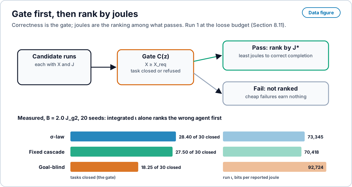
experiments/agency-run/results. A PNG copy is provided. Open full size · PNG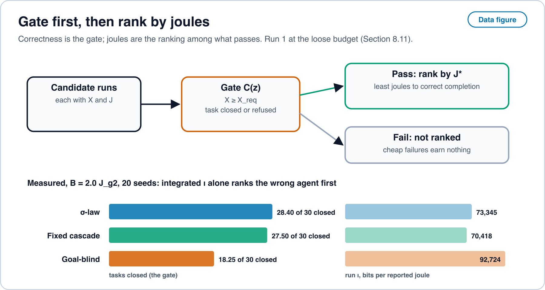
8.11.1 Second run: guarded acceptor, 40 seeds
This run is the same task class, the same gears and the same three arms as Section 8.11, on the same laptop. The preregistration for the second run was committed first (610dd4c). The pilot and the locked calibration came next (c88511f), and then the main run (920d7e2). Prediction 1 has no software analogue in this run: the agent has no declared act cost that falls with act time and no standing cost it controls, so the preregistration states that the dose-response design is not run.
Method.
- Guard. Every joule of an episode is charged inside the guard: selection, hash, gear steps, comparison, receipt and final read. The opening check uses spent . The law arms refuse when the guard fails. The goal-blind arm is cut.
- Refusal threshold. Both selectors use the -quantile of calibration costs for budget-fit tests. was locked from calibration replay before the main run: , with recall 1.0 and precision about 0.976 on the calibration split.
- Budgets and seeds. Per task, , the pilot median of g2 alone. Levels 0.5 and 1.0 bind: pilot fractions exceeding them are 0.98 and 0.4. Level 2.0 does not (0.0067). There are 40 seeds per condition. In all, 10,800 episodes ran.
- Quiet window. Quiet was not achieved. Probes ran until the limit. The last probe before the start, at 21:46 local time, recorded other-process CPU near 621% of one core, with mediaanalysisd and editor helpers at the top. Baseline package power was about 21.4 W. Package power in the main window was about 22.7 W. The run records
quiet_window = no. - Energy label. Every joule is
reported_j: the kernel’s per-process energy estimate for the agent (ri_energy_njfromproc_pid_rusage), with package figures from powermetrics where used for the cross-check.est_jis cycles times J, locked in the pilot.measured_jis empty: no wall meter was attached. - Package cross-check. In the main window the process meter read 42.35 J. Net package joules were 121.81 J, a ratio of about 2.88 to the process. Baseline package drift was about W. Because
quiet_window = no, the cross-check is declared not achievable. The per-process meter remains the run’s meter.
Results. Mean ± standard deviation over 40 seeds. A run is one arm at one budget level over all 30 tasks. CV is the coefficient of variation, standard deviation over mean. is reported in millijoules for comparison with Section 8.11.
| Arm | Tasks closed of 30 | (bits) | (reported, mJ) | (bits per reported joule) | CV of | Refusals | Cuts | Overspends | |
|---|---|---|---|---|---|---|---|---|---|
| σ-law | 0.5 | 0.62 ± 0.49 | 113 ± 89 | 59.5 ± 2.0 | 1,942 ± 1,525 | 0.785 | 29.38 | 0 | 0 |
| σ-law | 1.0 | 2.90 ± 1.74 | 523 ± 314 | 133.7 ± 13.8 | 4,150 ± 2,892 | 0.697 | 27.10 | 0 | 0 |
| σ-law | 2.0 | 22.73 ± 1.30 | 3,980 ± 206 | 197.3 ± 18.2 | 20,359 ± 2,388 | 0.117 | 7.28 | 0 | 0 |
| Fixed cascade (cheapest first) | 0.5 | 0.57 ± 0.50 | 104 ± 90 | 60.1 ± 2.1 | 1,777 ± 1,548 | 0.871 | 29.43 | 0 | 0 |
| Fixed cascade (cheapest first) | 1.0 | 2.67 ± 1.25 | 483 ± 226 | 140.3 ± 13.5 | 3,593 ± 1,948 | 0.542 | 27.32 | 0 | 0 |
| Fixed cascade (cheapest first) | 2.0 | 19.93 ± 1.42 | 3,509 ± 227 | 201.2 ± 20.4 | 17,684 ± 2,909 | 0.164 | 10.07 | 0 | 0 |
| Goal-blind | 0.5 | 0.12 ± 0.33 | 23 ± 61 | 35.4 ± 11.6 | 513 ± 1,397 | 2.723 | 0 | 22.85 | 0 |
| Goal-blind | 1.0 | 1.00 ± 0.93 | 181 ± 169 | 72.0 ± 19.5 | 2,661 ± 2,579 | 0.969 | 0 | 20.00 | 0 |
| Goal-blind | 2.0 | 10.65 ± 2.27 | 1,859 ± 400 | 97.3 ± 30.1 | 20,302 ± 5,766 | 0.284 | 0 | 8.70 | 0 |
- Per act. 7,960 acts ran. 2,448 were confirmed. Kendall’s tau-b between
est_jandreported_jwas 0.942 on 4,000 acts. The median act was about bits per reported joule. Every confirmed act sat far above per bit: the lowest was about times that floor. - Refusal. Recall was 1.0 on 49 infeasible pairs. There were 5,223 refusals. The share on tasks closed by some arm was about 0.081.
- Overspends. Zero episodes ended above budget. The maximum overspend fraction was : every episode finished under budget.
- Selectors, paired by seed. This analysis was declared in the preregistration. At the σ-law selector closed 2.8 more tasks per run than the fixed cascade (95% bootstrap interval 2.3 to 3.275). Its run was higher by 2,674 bits per joule (1,831 to 3,504). On 39 of 40 seeds the σ-law selector closed more. At and the intervals for the closed-task difference include zero. These results fire no falsifier.
Falsifier outcomes. All were fixed before the run. The table states the second-run outcome beside the first-run outcome.
| ID | Observation | Run 2 | Run 1 |
|---|---|---|---|
| R-F1 | At every binding level, the 95% interval of the paired per-task difference in median , σ-law minus fixed cascade, includes or exceeds zero | Held, because no interval could be formed: at no task closed by both, and at one did. Shared-task joules show no σ-law saving | Fired |
| R-F2 | Any episode ends above its budget | Held. 0 of 10,800. The guard charges comparison, receipt and final read | Fired |
| R-F3 | Refusal recall below 0.9 on infeasible pairs, or over 10% of refusals on pairs some arm closes | Held. Recall 1.0 on 49 infeasible pairs. Share on tasks closed by some arm about 0.081. The -quantile refusal threshold is the change from Run 1 | Fired |
| R-F4 | Kendall’s tau-b between est_j and reported_j per act below 0.8 | Held. 0.942 on 4,000 acts | Held |
| R-F5 | CV of run above 0.25 in any condition | Fired at binding levels (0.54 to 2.72) and for the goal-blind arm at (0.284). Held for both selectors at (0.117, 0.164) | Fired |
| R-F6 | Ranking by differs from ranking by integrated | Fired. At , ranks σ-law, fixed cascade, goal-blind. Integrated ranks σ-law, goal-blind, fixed cascade | Fired |
| R-F7 | A confirmed act below per bit | Held. The lowest act sat about times above | Held |
| R-F8 | Goal-blind run at least the better selector’s at a binding level | Held. 513 against 1,942 at . 2,661 against 4,150 at | Held |
What the run settles.
- The guard closes R-F2. Zero overspends.
- The refusal quantile closes R-F3. Recall stays 1.0 and the share of refusals on closable tasks falls under 10%.
- remains the ranking. Integrated still disagrees with it on the loose budget (R-F6).
- Run is still unstable across seeds at binding budgets (R-F5).
- R-F1 held only because too few tasks were closed by both selectors to form an interval. No run shows the σ-law selector closing a shared task in fewer joules. The paired-by-seed gain at is more closed tasks, not cheaper closures of the same tasks.
8.11.2 Second machine: a replication with a package energy counter
This run repeats the second-run protocol of Section 8.11.1 on a second machine with a different energy counter. It is a replication of the selector comparison, not a measurement of energy. Code, receipts and summaries are in experiments/agency-run: PREREGISTRATION_v2_jetson.md and its Amendment 1, results_jetson/summary.md (part A) and results_jetson_cyc/summary.md (part B). The preregistration addendum was committed first (cb059f0), then the meter backend and harness (1938577), then Amendment 1 (7703822). The part A pilot (6ddd086) and main run (a652503) came next, then the part B pilot (3fde1fb) and main run (1bb2444).
Method.
- Machine. A Linux laptop with a 14-core x86 processor: 6 performance cores with 2 threads each and 8 efficiency cores. Turbo was off. Every core was pinned to its base frequency: 2.6 GHz on performance cores and 1.9 GHz on efficiency cores. The agent ran pinned to one performance-core thread, one episode at a time. The median agent-core frequency during blocks was 2.6 GHz. The original settings were restored after the run.
- Unchanged. Tasks, predicate, coupled bits, gears g0 to g2, the three arms, the guard, the refusal replay, the budget levels , 40 seeds and 10,800 episodes per part, falsifiers R-F1 to R-F8 and the paired-by-seed analysis are those of Section 8.11.1.
- Energy counter. RAPL (Running Average Power Limit) is the processor’s on-chip package energy counter. Every interval was charged the package joules minus the idle baseline power of that block times the interval’s seconds. RAPL is a model and sensor inside the chip, not a wall meter. It counts every process on the package.
- Quiet window. Quiet was not achieved:
quiet_window = no. A CI (continuous integration) runner built Rust code on the machine throughout. The 40 probes before the start saw other processes using from 1.0 to 20.0 cores and package power from 2.3 to 28.7 W. The per-block gate was met before 180 of 360 blocks in part A and 244 of 360 in part B. 98 and 208 blocks were quiet for their whole length. - Part A. The agent’s meter is RAPL read before and after each act. Every figure is
reported_j. - Part B. Amendment 1 added this part before any pilot, because a harness test showed that acts last about 0.01 to 6 ms while RAPL updates about every 1 ms in steps of about 5 to 60 mJ. The agent’s meter is
est_j: the agent thread’s user cycles times . was calibrated on RAPL in the part B pilot, net of idle, over 8 rounds of 3 s, on the second attempt: J per cycle, from 41.11 J of net package energy over 62,516,635,701 cycles. Every part B joule figure isest_j. RAPL figures logged beside it stayreported_j. - Labels.
measured_jis empty in both parts. No wall meter or shunt meter was attached. - Arm names. Arm names and their code fields follow Section 8.3. The goal-blind baseline is
blind.
Part A results: RAPL read per act. Mean ± standard deviation over 40 seeds. is reported_j in joules, as in the summary. Levels 0.5, 1.0 and 2.0 all bind: 0.647, 0.40 and 0.353 of pilot g2 runs exceed them.
| Arm | Tasks closed of 30 | (bits) | (reported, J) | (bits per reported joule) | CV of | Refusals | Cuts | Overspends | |
|---|---|---|---|---|---|---|---|---|---|
| σ-law | 0.5 | 0.00 | 0 | 0.0018 | 0 | n/a | 30.00 | 0.00 | 323 |
| σ-law | 1.0 | 0.00 | 0 | 0.0002 | 0 | n/a | 30.00 | 0.00 | 322 |
| σ-law | 2.0 | 1.00 ± 0.39 | 181 ± 71 | 0.0018 ± 0.0336 | 14,427 ± 18,680 | 1.295 | 29.00 | 0.00 | 322 |
| Fixed cascade (cheapest first) | 0.5 | 0.00 | 0 | -0.0008 | 0 | n/a | 30.00 | 0.00 | 326 |
| Fixed cascade (cheapest first) | 1.0 | 0.00 | 0 | -0.0005 | 0 | n/a | 30.00 | 0.00 | 324 |
| Fixed cascade (cheapest first) | 2.0 | 1.00 ± 0.51 | 181 ± 91 | 0.0107 ± 0.0286 | 15,451 ± 23,767 | 1.538 | 29.00 | 0.00 | 320 |
| Goal-blind | 0.5 | 0.00 | 0 | 0.0026 | 0 | n/a | 0.00 | 30.00 | 327 |
| Goal-blind | 1.0 | 0.00 | 0 | 0.0009 | 0 | n/a | 0.00 | 30.00 | 323 |
| Goal-blind | 2.0 | 0.28 ± 0.45 | 50 ± 82 | 0.0019 ± 0.0180 | 3,801 ± 13,749 | 3.618 | 0.00 | 28.90 | 321 |
- Counter resolution. The median episode lasted about 0.04 ms. 10,075 of 10,800 episodes saw no change in the package counter. 10,549 had
reported_jat or below zero after idle subtraction. - Budgets. Pilot medians of ranged from to J, median J. The guard’s open threshold was 0.117 J. Budgets fell below it for 30, 30 and 28 of 30 tasks at the three levels, so the law arms refused nearly every task.
- Overspends. Every condition recorded 320 to 327 overspends. The maximum overspend fraction was 10.86. A charge that reads zero for most acts and one whole counter step for a few cannot hold a budget of a few millijoules.
- Per act. 137 acts ran. 91 were confirmed. 44 acts read zero. 26 confirmed acts read zero or less. Kendall’s tau-b between
est_jandreported_jwas 0.368 on 93 acts. - Cross-check. Block package net was 3.445 J against 2.737 J summed over episodes, a ratio of 0.794. Idle package power was 4.01 W before the run and 5.55 W after. The cross-check is declared not achievable.
- Selectors, paired by seed. At the closed-task difference was 0 (95% bootstrap interval to ). The run difference was 1,328 bits per reported joule ( to ). 30 of 40 seeds tied. At 0.5 and 1.0 no arm closed a task.
Part B results: cycle count times a RAPL-calibrated constant. Mean ± standard deviation over 40 seeds. is est_j in joules, as in the summary. Levels 0.5 and 1.0 bind: 0.98 and 0.40 of pilot g2 runs exceed them. Level 2.0 does not (0.0).
| Arm | Tasks closed of 30 | (bits) | (estimated, J) | (bits per estimated joule) | CV of | Refusals | Cuts | Overspends | |
|---|---|---|---|---|---|---|---|---|---|
| σ-law | 0.5 | 1.10 ± 0.98 | 200 ± 178 | 0.0345 ± 0.0017 | 6,027 ± 5,458 | 0.906 | 28.90 | 0.00 | 0 |
| σ-law | 1.0 | 8.75 ± 3.14 | 1,574 ± 565 | 0.0805 ± 0.0098 | 20,519 ± 8,516 | 0.415 | 21.25 | 0.00 | 0 |
| σ-law | 2.0 | 28.60 ± 0.98 | 4,882 ± 154 | 0.1008 ± 0.0234 | 50,667 ± 10,088 | 0.199 | 1.40 | 0.00 | 0 |
| Fixed cascade (cheapest first) | 0.5 | 1.15 ± 0.92 | 208 ± 167 | 0.0366 ± 0.0013 | 5,833 ± 4,757 | 0.816 | 28.85 | 0.00 | 0 |
| Fixed cascade (cheapest first) | 1.0 | 9.22 ± 3.07 | 1,660 ± 551 | 0.0813 ± 0.0106 | 21,412 ± 8,130 | 0.380 | 20.77 | 0.00 | 0 |
| Fixed cascade (cheapest first) | 2.0 | 27.77 ± 2.30 | 4,745 ± 377 | 0.1099 ± 0.0339 | 47,108 ± 13,216 | 0.281 | 2.23 | 0.00 | 0 |
| Goal-blind | 0.5 | 0.20 ± 0.46 | 36 ± 84 | 0.0210 ± 0.0055 | 1,722 ± 3,927 | 2.280 | 0.00 | 21.50 | 0 |
| Goal-blind | 1.0 | 3.73 ± 2.12 | 667 ± 381 | 0.0436 ± 0.0140 | 16,393 ± 9,246 | 0.564 | 0.00 | 16.68 | 0 |
| Goal-blind | 2.0 | 15.65 ± 2.50 | 2,662 ± 433 | 0.0499 ± 0.0160 | 57,266 ± 14,596 | 0.255 | 0.00 | 4.17 | 0 |
- Per act. 7,800 acts ran. 3,847 were confirmed. The median act was 69,892 bits per estimated joule, with interquartile range 35,759 to 146,697. Every confirmed act sat far above per bit: the lowest was about times that floor, the median about times.
- Refusal. Recall was 1.0 on 45 infeasible pairs. There were 4,136 refusals. The share on tasks closed by some arm was about 0.071.
- Overspends. Zero episodes ended above budget. The maximum overspend fraction was .
- Shared tasks. At , 9 tasks closed by both selectors. The paired per-task difference in median , σ-law minus fixed cascade, had mean J (95% interval to , Wilcoxon ). At one task closed by both, with difference J. At , 29 tasks closed by both, with mean difference J ( to , ).
- Selectors, paired by seed. At the σ-law selector closed 0.825 more tasks per run than the fixed cascade (95% bootstrap interval 0.125 to 1.575). Its run was higher by 3,559 bits per estimated joule ( to ). 9 of 40 seeds favored the σ-law selector and 27 tied. At the closed-task difference was ( to ). At it was ( to ).
- The estimate against the counter. Kendall’s tau-b between each episode’s
est_jand the same episode’s RAPL package net was on 4,000 episodes. 5,258 of 10,800 episodes saw no change in the package counter. Summed over blocks,est_jwas 23.23 J against 17.14 J of RAPL package net, a ratio of 1.355. Idle package power was 9.37 W before the run and 3.17 W after. The cross-check is declared not achievable.
Falsifier outcomes. All were fixed before the run. Part B replaces R-F4 with the episode test against RAPL, as Amendment 1 states. In Run 2 and in the two parts here, “Held” means the observation did not occur.
| ID | Observation | Part A (RAPL per act) | Part B (cycle model) | Run 2 |
|---|---|---|---|---|
| R-F1 | At every binding level, the 95% interval of the paired per-task difference in median , σ-law minus fixed cascade, includes or exceeds zero | Held, because no interval could be formed: one task closed by both, at , with difference J, and none at the other levels | Held, because the observation needs every binding level and has a single shared task ( J) and no interval. At the interval includes zero | Held |
| R-F2 | Any episode ends above its budget | Fired. 320 to 327 per condition | Held. 0 of 10,800 | Held |
| R-F3 | Refusal recall below 0.9 on infeasible pairs, or over 10% of refusals on pairs some arm closes | Held. Recall 1.0 on 88 pairs. Share 0.0011 | Held. Recall 1.0 on 45 pairs. Share 0.071 | Held |
| R-F4 | Part A: Kendall’s tau-b between est_j and reported_j per act below 0.8. Part B: tau-b between episode est_j and episode RAPL net below 0.8 | Fired. 0.368 on 93 acts | Fired. on 4,000 episodes | Held |
| R-F5 | CV of run above 0.25 in any condition | Fired (1.295 to 3.618) | Fired. 0.380 to 2.280 at binding levels. At : σ-law 0.199, fixed cascade 0.281, goal-blind 0.255 | Fired |
| R-F6 | Ranking by differs from ranking by integrated | Fired. At , ranks σ-law, fixed cascade, goal-blind. Integrated ranks fixed cascade first | Fired. At , ranks σ-law, fixed cascade, goal-blind. Integrated ranks goal-blind, σ-law, fixed cascade | Fired |
| R-F7 | A confirmed act below per bit | Fired. 26 confirmed acts read zero or less, which places them below the floor. That is counter quantization | Held. The lowest act sat about times above | Held |
| R-F8 | Goal-blind run at least the better selector’s at a binding level | Fired. At and every arm reads 0 | Held. 1,722 against 6,027 at . 16,393 against 21,412 at | Held |
What the replication settles.
- Per-act RAPL cannot meter acts shorter than one millisecond. Most episodes saw no counter update, so the guard refused or overspent from quantization alone. Part A is a meter-resolution result. It says nothing about the selectors.
- With a cycle meter, the selection result has the same sign as Run 2 at : the σ-law selector closed more tasks per run. The gain is smaller (0.825 against 2.8), and level 2.0 did not bind on this machine. At the binding levels the intervals include zero.
- The cycle model did not track the package counter episode by episode (tau-b ), and its block total was 1.355 times the counter’s net. Part B joules rank acts by cycles. They are not energy readings.
- Shared-task joules show no σ-law saving here either. Where the σ-law selector gains, it gains in tasks closed, not in cheaper closure of the same task.
- No figure in this section is
measured_j.
Figure 5 sets the closed-task results of the three runs side by side.
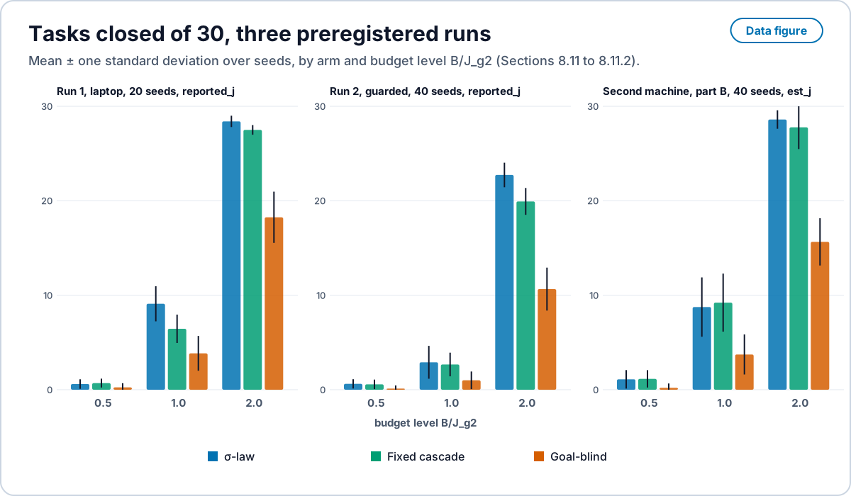
experiments/agency-run/results, results2 and results_jetson_cyc. A PNG copy is provided. Open full size · PNG
What replicates, and what does not. The run 1 selector result was exploratory. Two later runs tested it under preregistration.
| Claim from run 1 (exploratory) | Run 2 (preregistered) | Second machine, part B (preregistered) |
|---|---|---|
| More tasks closed at : +2.65 (1.5 to 3.8) | Not replicated. The interval includes zero | Not replicated. ( to ) |
| More tasks closed at : +0.9 (0.55 to 1.25) | Replicated. +2.8 (2.3 to 3.275) | Replicated. +0.825 (0.125 to 1.575) |
| Joules per closed task | Equal. No shared-task saving | Equal. Shared-task intervals include zero |
The replicated result is narrow. At the loosest budget level the σ-law selector closes more tasks than the fixed cascade, on two machines. No run shows fewer joules for the same closed task, and the binding-budget gain of run 1 did not replicate. Part A is a meter-resolution result and tests neither claim.
Measurement protocol for the next run. Both parts fail at the meter, so the protocol changes before the selectors are tested again.
- Idle machine. Stop nothing that belongs to someone else. Wait for a quiet window, or schedule one: other processes at or below 0.5 cores for the whole run, with
quiet_window = yesrecorded. If quiet is not reached, the run does not start. - Wall or shunt meter. Attach a wall power meter, or a shunt meter on the supply rail, sampled faster than one act. Only its readings fill
measured_j. - Resolution check first. Before the pilot, record the meter’s update interval and step size against the median act length. If the meter cannot resolve one act, meter blocks of acts and attribute by count, and say so in the preregistration.
- Calibrate the estimate on the meter. Fit
est_jon the wall or shunt meter at block level, and require R-F4 to hold beforeest_jdrives the guard. - Pin and record. Pin frequency, record idle baselines before and after, report drift, and keep the package counter as a labeled cross-check.
- Task closure is primary. The next run’s preregistration makes task closure the primary endpoint: the paired-by-seed difference in tasks closed, σ-law minus fixed cascade, at each budget level, with the Holm step-down correction across levels. Shared-task joules (R-F1) are secondary.
8.12 Reporting
Publish all receipts, raw meter traces, idle baselines and analysis code with the result. Report measured, reported and estimated joules in separate columns. Never sum across tiers. State which falsifiers fired, with the same prominence as those that passed. Every run also answers the checklist of Takahashi and Hayashi [239]: the accounting boundary; the energy balance terms (stored energy and exported work, or a statement that they are negligible); the baseline and whether joules are total or incremental; the coarse-graining of outcomes; the horizon and reset protocol; wall-clock time and mean power beside bits per joule; and the estimator of coupled bits with its bias correction.
References
Entries marked “preprint” are cited by their arXiv posting. Entries published in a language other than English say so.
- Pearl, J. (1995). Causal diagrams for empirical research. Biometrika 82:669-688. https://doi.org/10.1093/biomet/82.4.669
- Everitt, T., Hutter, M., Kumar, R. and Krakovna, V. (2019). Reward tampering problems and solutions in reinforcement learning: a causal influence diagram perspective. arXiv:1908.04734 (preprint).
- Sagawa, T. and Ueda, M. (2008). Second law of thermodynamics with discrete quantum feedback control. Physical Review Letters 100:080403. https://doi.org/10.1103/PhysRevLett.100.080403
- Sagawa, T. and Ueda, M. (2010). Generalized Jarzynski equality under nonequilibrium feedback control. Physical Review Letters 104:090602. https://doi.org/10.1103/PhysRevLett.104.090602
- Sagawa, T. and Ueda, M. (2009). Minimal energy cost for thermodynamic information processing: measurement and information erasure. Physical Review Letters 102:250602. https://doi.org/10.1103/PhysRevLett.102.250602
- Landauer, R. (1961). Irreversibility and heat generation in the computing process. IBM Journal of Research and Development 5:183-191. https://doi.org/10.1147/rd.53.0183
- Bennett, C. H. (1982). The thermodynamics of computation: a review. International Journal of Theoretical Physics 21:905-940. https://doi.org/10.1007/BF02084158
- Ay, N. and Polani, D. (2008). Information flows in causal networks. Advances in Complex Systems 11:17-41. https://doi.org/10.1142/S0219525908001465
- Klyubin, A. S., Polani, D. and Nehaniv, C. L. (2005). Empowerment: a universal agent-centric measure of control. 2005 IEEE Congress on Evolutionary Computation 1:128-135. https://doi.org/10.1109/CEC.2005.1554676
- Kenton, Z., Kumar, R., Farquhar, S., Richens, J. et al. (2023). Discovering agents. Artificial Intelligence 322:103963. https://doi.org/10.1016/j.artint.2023.103963
- James, R. G., Barnett, N. and Crutchfield, J. P. (2016). Information flows? A critique of transfer entropies. Physical Review Letters 116:238701. https://doi.org/10.1103/PhysRevLett.116.238701
- Lizier, J. T. and Prokopenko, M. (2010). Differentiating information transfer and causal effect. The European Physical Journal B 73:605-615. https://doi.org/10.1140/epjb/e2010-00034-5
- Janzing, D., Balduzzi, D., Grosse-Wentrup, M. and Schölkopf, B. (2013). Quantifying causal influences. The Annals of Statistics 41. https://doi.org/10.1214/13-AOS1145
- Albantakis, L., Marshall, W., Hoel, E. and Tononi, G. (2019). What caused what? A quantitative account of actual causation using dynamical causal networks. Entropy 21:459. https://doi.org/10.3390/e21050459
- Aguilera, M., Millidge, B., Tschantz, A. and Buckley, C. L. (2022). How particular is the physics of the free energy principle? Physics of Life Reviews 40:24-50. https://doi.org/10.1016/j.plrev.2021.11.001
- Biehl, M., Pollock, F. A. and Kanai, R. (2021). A technical critique of some parts of the free energy principle. Entropy 23:293. https://doi.org/10.3390/e23030293
- Bruineberg, J., Dołęga, K., Dewhurst, J. and Baltieri, M. (2022). The emperor’s new Markov blankets. Behavioral and Brain Sciences 45:e183. https://doi.org/10.1017/S0140525X21002351
- Orseau, L., McGregor McGill, S. and Legg, S. (2018). Agents and devices: a relative definition of agency. arXiv:1805.12387 (preprint).
- Albantakis, L., Barbosa, L., Findlay, G., Grasso, M. et al. (2023). Integrated information theory (IIT) 4.0: formulating the properties of phenomenal existence in physical terms. PLOS Computational Biology 19:e1011465. https://doi.org/10.1371/journal.pcbi.1011465
- Krakauer, D., Bertschinger, N., Olbrich, E., Flack, J. C. and Ay, N. (2020). The information theory of individuality. Theory in Biosciences 139:209-223. https://doi.org/10.1007/s12064-020-00313-7
- Hoel, E. P., Albantakis, L. and Tononi, G. (2013). Quantifying causal emergence shows that macro can beat micro. Proceedings of the National Academy of Sciences 110:19790-19795. https://doi.org/10.1073/pnas.1314922110
- Rosas, F. E., Mediano, P. A. M., Biehl, M., Chandaria, S. and Polani, D. (2020). Causal blankets: theory and algorithmic framework. In Active Inference: IWAI 2020, Communications in Computer and Information Science, Springer, pp. 187-198. https://doi.org/10.1007/978-3-030-64919-7_19
- Shiraishi, N., Funo, K. and Saito, K. (2018). Speed limit for classical stochastic processes. Physical Review Letters 121:070601. https://doi.org/10.1103/PhysRevLett.121.070601
- Esposito, M. and Van den Broeck, C. (2011). Second law and Landauer principle far from equilibrium. EPL 95:40004. https://doi.org/10.1209/0295-5075/95/40004
- Barato, A. C. and Seifert, U. (2015). Thermodynamic uncertainty relation for biomolecular processes. Physical Review Letters 114:158101. https://doi.org/10.1103/PhysRevLett.114.158101
- Gingrich, T. R., Horowitz, J. M., Perunov, N. and England, J. L. (2016). Dissipation bounds all steady-state current fluctuations. Physical Review Letters 116:120601. https://doi.org/10.1103/PhysRevLett.116.120601
- Paneru, G., Dutta, S., Tlusty, T. and Pak, H. K. (2020). Reaching and violating thermodynamic uncertainty bounds in information engines. Physical Review E 102:032126. https://doi.org/10.1103/PhysRevE.102.032126
- Potts, P. P. and Samuelsson, P. (2019). Thermodynamic uncertainty relations including measurement and feedback. Physical Review E 100:052137. https://doi.org/10.1103/PhysRevE.100.052137
- Proesmans, K., Ehrich, J. and Bechhoefer, J. (2020). Finite-time Landauer principle. Physical Review Letters 125:100602. https://doi.org/10.1103/PhysRevLett.125.100602
- Sivak, D. A. and Crooks, G. E. (2012). Thermodynamic metrics and optimal paths. Physical Review Letters 108:190602. https://doi.org/10.1103/PhysRevLett.108.190602
- Margolus, N. and Levitin, L. B. (1998). The maximum speed of dynamical evolution. Physica D 120:188-195. https://doi.org/10.1016/S0167-2789(98)00054-2
- Touchette, H. and Lloyd, S. (2000). Information-theoretic limits of control. Physical Review Letters 84:1156-1159. https://doi.org/10.1103/PhysRevLett.84.1156
- Touchette, H. and Lloyd, S. (2004). Information-theoretic approach to the study of control systems. Physica A 331:140-172. https://doi.org/10.1016/j.physa.2003.09.007
- Garrahan, J. P. (2017). Simple bounds on fluctuations and uncertainty relations for first-passage times of counting observables. Physical Review E 95:032134. https://doi.org/10.1103/PhysRevE.95.032134
- Bennett, C. H. (1973). Logical reversibility of computation. IBM Journal of Research and Development 17:525-532. https://doi.org/10.1147/rd.176.0525
- Sagawa, T. and Ueda, M. (2012). Fluctuation theorem with information exchange: role of correlations in stochastic thermodynamics. Physical Review Letters 109:180602. https://doi.org/10.1103/PhysRevLett.109.180602
- Hartle, H., Wolpert, D., Stier, A., Kempes, C. P. and Manzano, G. (2024). Work extraction with feedback control using limited resources. arXiv:2407.05507 (preprint).
- Horodecki, M. and Oppenheim, J. (2013). Fundamental limitations for quantum and nanoscale thermodynamics. Nature Communications 4:2059. https://doi.org/10.1038/ncomms3059
- Parrondo, J. M. R., Horowitz, J. M. and Sagawa, T. (2015). Thermodynamics of information. Nature Physics 11:131-139. https://doi.org/10.1038/nphys3230
- Seifert, U. (2012). Stochastic thermodynamics, fluctuation theorems and molecular machines. Reports on Progress in Physics 75:126001. https://doi.org/10.1088/0034-4885/75/12/126001
- Conant, R. C. and Ashby, W. R. (1970). Every good regulator of a system must be a model of that system. International Journal of Systems Science 1:89-97. https://doi.org/10.1080/00207727008920220
- Richens, J. and Everitt, T. (2024). Robust agents learn causal world models. International Conference on Learning Representations (ICLR 2024), oral, honorable mention. arXiv:2402.10877.
- Richens, J., Abel, D., Bellot, A. and Everitt, T. (2025). General agents contain world models. arXiv:2506.01622 (preprint).
- Horowitz, J. M. and Esposito, M. (2014). Thermodynamics with continuous information flow. Physical Review X 4:031015. https://doi.org/10.1103/PhysRevX.4.031015
- Ito, S. and Sagawa, T. (2013). Information thermodynamics on causal networks. Physical Review Letters 111:180603. https://doi.org/10.1103/PhysRevLett.111.180603
- Hartich, D., Barato, A. C. and Seifert, U. (2014). Stochastic thermodynamics of bipartite systems: transfer entropy inequalities and a Maxwell’s demon interpretation. Journal of Statistical Mechanics P02016. https://doi.org/10.1088/1742-5468/2014/02/P02016
- Allahverdyan, A. E., Janzing, D. and Mahler, G. (2009). Thermodynamic efficiency of information and heat flow. Journal of Statistical Mechanics P09011. https://doi.org/10.1088/1742-5468/2009/09/P09011
- Esposito, M. and Schaller, G. (2012). Stochastic thermodynamics for “Maxwell demon” feedbacks. EPL 99:30003. https://doi.org/10.1209/0295-5075/99/30003
- Mandal, D. and Jarzynski, C. (2012). Work and information processing in a solvable model of Maxwell’s demon. PNAS 109:11641-11645. https://doi.org/10.1073/pnas.1204263109
- Boyd, A. B., Mandal, D. and Crutchfield, J. P. (2016). Identifying functional thermodynamics in autonomous Maxwellian ratchets. New Journal of Physics 18:023049. https://doi.org/10.1088/1367-2630/18/2/023049
- Boyd, A. B., Mandal, D. and Crutchfield, J. P. (2018). Thermodynamics of modularity: structural costs beyond the Landauer bound. Physical Review X 8:031036. https://doi.org/10.1103/PhysRevX.8.031036
- Wolpert, D. H. and Kolchinsky, A. (2020). Thermodynamics of computing with circuits. New Journal of Physics 22:063047. https://doi.org/10.1088/1367-2630/ab82b8
- Kolchinsky, A. and Wolpert, D. H. (2017). Dependence of dissipation on the initial distribution over states. Journal of Statistical Mechanics 083202. https://doi.org/10.1088/1742-5468/aa7ee1
- Still, S., Sivak, D. A., Bell, A. J. and Crooks, G. E. (2012). Thermodynamics of prediction. Physical Review Letters 109:120604. https://doi.org/10.1103/PhysRevLett.109.120604
- Kolchinsky, A. and Wolpert, D. H. (2018). Semantic information, autonomous agency and non-equilibrium statistical physics. Interface Focus 8:20180041. https://doi.org/10.1098/rsfs.2018.0041
- Ortega, P. A. and Braun, D. A. (2013). Thermodynamics as a theory of decision-making with information-processing costs. Proceedings of the Royal Society A 469:20120683. https://doi.org/10.1098/rspa.2012.0683
- Kolchinsky, A. and Wolpert, D. H. (2020). Thermodynamic costs of Turing machines. Physical Review Research 2:033312. https://doi.org/10.1103/PhysRevResearch.2.033312
- Kolchinsky, A. and Wolpert, D. H. (2021). Work, entropy production, and thermodynamics of information under protocol constraints. Physical Review X 11:041024. https://doi.org/10.1103/PhysRevX.11.041024
- Manzano, G., Kardeş, G., Roldán, É. and Wolpert, D. H. (2024). Thermodynamics of computations with absolute irreversibility, unidirectional transitions, and stochastic computation times. Physical Review X 14:021026. https://doi.org/10.1103/PhysRevX.14.021026
- Bérut, A., Arakelyan, A., Petrosyan, A., Ciliberto, S., Dillenschneider, R. and Lutz, E. (2012). Experimental verification of Landauer’s principle linking information and thermodynamics. Nature 483:187-189. https://doi.org/10.1038/nature10872
- Jun, Y., Gavrilov, M. and Bechhoefer, J. (2014). High-precision test of Landauer’s principle in a feedback trap. Physical Review Letters 113:190601. https://doi.org/10.1103/PhysRevLett.113.190601
- Orlov, A. O., Lent, C. S., Thorpe, C. C., Boechler, G. P. and Snider, G. L. (2012). Experimental test of Landauer’s principle at the sub-k_BT level. Japanese Journal of Applied Physics 51:06FE10. https://doi.org/10.1143/JJAP.51.06FE10
- Hong, J., Lambson, B., Dhuey, S. and Bokor, J. (2016). Experimental test of Landauer’s principle in single-bit operations on nanomagnetic memory bits. Science Advances 2:e1501492. https://doi.org/10.1126/sciadv.1501492
- Gavrilov, M. and Bechhoefer, J. (2016). Erasure without work in an asymmetric double-well potential. Physical Review Letters 117:200601. https://doi.org/10.1103/PhysRevLett.117.200601
- Gavrilov, M., Chétrite, R. and Bechhoefer, J. (2017). Direct measurement of weakly nonequilibrium system entropy is consistent with Gibbs-Shannon form. PNAS 114:11097-11102. https://doi.org/10.1073/pnas.1708689114
- Yan, L. L., Xiong, T. P., Rehan, K., Zhou, F., Liang, D. F. et al. (2018). Single-atom demonstration of the quantum Landauer principle. Physical Review Letters 120:210601. https://doi.org/10.1103/PhysRevLett.120.210601
- Dago, S., Pereda, J., Barros, N., Ciliberto, S. and Bellon, L. (2021). Information and thermodynamics: fast and precise approach to Landauer’s bound in an underdamped micromechanical oscillator. Physical Review Letters 126:170601. https://doi.org/10.1103/PhysRevLett.126.170601
- Scandi, M., Barker, D., Lehmann, S., Dick, K. A., Maisi, V. F. and Perarnau-Llobet, M. (2022). Minimally dissipative information erasure in a quantum dot via thermodynamic length. Physical Review Letters 129:270601. https://doi.org/10.1103/PhysRevLett.129.270601
- Toyabe, S., Sagawa, T., Ueda, M., Muneyuki, E. and Sano, M. (2010). Experimental demonstration of information-to-energy conversion and validation of the generalized Jarzynski equality. Nature Physics 6:988-992. https://doi.org/10.1038/nphys1821
- Koski, J. V., Maisi, V. F., Pekola, J. P. and Averin, D. V. (2014). Experimental realization of a Szilard engine with a single electron. PNAS 111:13786-13789. https://doi.org/10.1073/pnas.1406966111
- Koski, J. V., Maisi, V. F., Sagawa, T. and Pekola, J. P. (2014). Experimental observation of the role of mutual information in the nonequilibrium dynamics of a Maxwell demon. Physical Review Letters 113:030601. https://doi.org/10.1103/PhysRevLett.113.030601
- Koski, J. V., Kutvonen, A., Khaymovich, I. M., Ala-Nissila, T. and Pekola, J. P. (2015). On-chip Maxwell’s demon as an information-powered refrigerator. Physical Review Letters 115:260602. https://doi.org/10.1103/PhysRevLett.115.260602
- Camati, P. A., Peterson, J. P. S., Batalhão, T. B., Micadei, K., Souza, A. M. et al. (2016). Experimental rectification of entropy production by Maxwell’s demon in a quantum system. Physical Review Letters 117:240502. https://doi.org/10.1103/PhysRevLett.117.240502
- Peterson, J. P. S., Sarthour, R. S., Souza, A. M., Oliveira, I. S., Goold, J. et al. (2016). Experimental demonstration of information to energy conversion in a quantum system at the Landauer limit. Proceedings of the Royal Society A 472:20150813. https://doi.org/10.1098/rspa.2015.0813
- Cottet, N., Jezouin, S., Bretheau, L., Campagne-Ibarcq, P., Ficheux, Q. et al. (2017). Observing a quantum Maxwell demon at work. PNAS 114:7561-7564. https://doi.org/10.1073/pnas.1704827114
- Masuyama, Y., Funo, K., Murashita, Y., Noguchi, A., Kono, S. et al. (2018). Information-to-work conversion by Maxwell’s demon in a superconducting circuit quantum electrodynamical system. Nature Communications 9:1291. https://doi.org/10.1038/s41467-018-03686-y
- Naghiloo, M., Alonso, J. J., Romito, A., Lutz, E. and Murch, K. W. (2018). Information gain and loss for a quantum Maxwell’s demon. Physical Review Letters 121:030604. https://doi.org/10.1103/PhysRevLett.121.030604
- Kumar, A., Wu, T.-Y., Giraldo, F. and Weiss, D. S. (2018). Sorting ultracold atoms in a three-dimensional optical lattice in a realization of Maxwell’s demon. Nature 561:83-87. https://doi.org/10.1038/s41586-018-0458-7
- Linpeng, X., Bresque, L., Maffei, M., Jordan, A. N. et al. (2022). Energetic cost of measurements using quantum, coherent, and thermal light. Physical Review Letters 128:220506. https://doi.org/10.1103/PhysRevLett.128.220506
- Paneru, G., Lee, D. Y., Tlusty, T. and Pak, H. K. (2018). Lossless Brownian information engine. Physical Review Letters 120:020601. https://doi.org/10.1103/PhysRevLett.120.020601
- Admon, T., Rahav, S. and Roichman, Y. (2018). Experimental realization of an information machine with tunable temporal correlations. Physical Review Letters 121:180601. https://doi.org/10.1103/PhysRevLett.121.180601
- Ribezzi-Crivellari, M. and Ritort, F. (2019). Large work extraction and the Landauer limit in a continuous Maxwell demon. Nature Physics 15:660-664. https://doi.org/10.1038/s41567-019-0481-0
- Debiossac, M., Grass, D., Alonso, J. J., Lutz, E. and Kiesel, N. (2020). Thermodynamics of continuous non-Markovian feedback control. Nature Communications 11:1360. https://doi.org/10.1038/s41467-020-15148-5
- Saha, T. K., Lucero, J. N. E., Ehrich, J., Sivak, D. A. and Bechhoefer, J. (2021). Maximizing power and velocity of an information engine. PNAS 118:e2023356118. https://doi.org/10.1073/pnas.2023356118
- Saha, T. K., Lucero, J. N. E., Ehrich, J., Sivak, D. A. and Bechhoefer, J. (2022). Bayesian information engine that optimally exploits noisy measurements. Physical Review Letters 129:130601. https://doi.org/10.1103/PhysRevLett.129.130601
- Saha, T. K., Ehrich, J., Gavrilov, M., Still, S., Sivak, D. A. and Bechhoefer, J. (2023). Information engine in a nonequilibrium bath. Physical Review Letters 131:057101. https://doi.org/10.1103/PhysRevLett.131.057101
- Barker, D., Scandi, M., Lehmann, S., Thelander, C., Dick, K. A., Perarnau-Llobet, M. and Maisi, V. F. (2022). Experimental verification of the work fluctuation-dissipation relation for information-to-work conversion. Physical Review Letters 128:040602. https://doi.org/10.1103/PhysRevLett.128.040602
- Yan, L.-L., Bu, J.-T., Zeng, Q., Zhang, K., Cui, K.-F. et al. (2024). Experimental verification of demon-involved fluctuation theorems. Physical Review Letters 133:090402. https://doi.org/10.1103/PhysRevLett.133.090402
- Zeng, Q. and Wang, J. (2021). New fluctuation theorems on Maxwell’s demon. Science Advances 7:eabf1807. https://doi.org/10.1126/sciadv.abf1807
- Demin, A. V. and Vityaev, E. E. (2014). Learning in a virtual model of the C. elegans nematode for locomotion and chemotaxis. Biologically Inspired Cognitive Architectures 7:9-14. https://doi.org/10.1016/j.bica.2013.11.005
- Putintsev, N. I., Isupov, O. V. and Vityaev, E. E. (2015). Adaptive control system for a mobile agent in a physical environment based on functional systems theory. Russian Journal of Genetics: Applied Research 5:601-608. https://doi.org/10.1134/S2079059715060131
- Rosenblueth, A., Wiener, N. and Bigelow, J. (1943). Behavior, purpose and teleology. Philosophy of Science 10:18-24. https://doi.org/10.1086/286788
- Anokhin, P. K. (1968). The functional system as a unit of organism integrative activity. In Systems Theory and Biology, Springer, pp. 376-403. https://doi.org/10.1007/978-3-642-88343-9_15
- Anokhin, P. K. (1974). The biological roots of the conditioned reflex. In Biology and Neurophysiology of the Conditioned Reflex and Its Role in Adaptive Behavior, Pergamon, pp. 1-24. https://doi.org/10.1016/B978-0-08-021516-7.50008-2
- Sudakov, K. V. (1997). The theory of functional systems: general postulates and principles of dynamic organization. Integrative Physiological and Behavioral Science 32:392-414. https://doi.org/10.1007/BF02688634
- Shvyrkov, V. B. (1980). Goal as a system-forming factor in behavior and learning. In Neural Mechanisms of Goal-directed Behavior and Learning, Academic Press, pp. 199-219. https://doi.org/10.1016/B978-0-12-688980-2.50018-7
- Rosen, R. (2012). Anticipatory Systems: Philosophical, Mathematical, and Methodological Foundations, 2nd ed. Springer. https://doi.org/10.1007/978-1-4614-1269-4
- Sterling, P. (2012). Allostasis: a model of predictive regulation. Physiology & Behavior 106:5-15. https://doi.org/10.1016/j.physbeh.2011.06.004
- Virgo, N., Biehl, M. and McGregor, S. (2021). Interpreting dynamical systems as Bayesian reasoners. In Machine Learning and Principles and Practice of Knowledge Discovery in Databases (ECML PKDD 2021 workshops), Communications in Computer and Information Science, Springer, pp. 726-762. https://doi.org/10.1007/978-3-030-93736-2_52
- Biehl, M. and Virgo, N. (2023). Interpreting systems as solving POMDPs: a step towards a formal understanding of agency. In Active Inference: IWAI 2022, Communications in Computer and Information Science 1721, Springer, pp. 16-31. https://doi.org/10.1007/978-3-031-28719-0_2
- Maturana, H. R. and Varela, F. J. (1980). Autopoiesis and Cognition: The Realization of the Living. Reidel. https://doi.org/10.1007/978-94-009-8947-4
- Kauffman, S. (2003). Molecular autonomous agents. Philosophical Transactions of the Royal Society A 361:1089-1099. https://doi.org/10.1098/rsta.2003.1186
- Di Paolo, E. A. (2005). Autopoiesis, adaptivity, teleology, agency. Phenomenology and the Cognitive Sciences 4:429-452. https://doi.org/10.1007/s11097-005-9002-y
- Barandiaran, X. and Moreno, A. (2006). On what makes certain dynamical systems cognitive: a minimally cognitive organization program. Adaptive Behavior 14:171-185. https://doi.org/10.1177/105971230601400208
- Barandiaran, X. and Moreno, A. (2008). Adaptivity: from metabolism to behavior. Adaptive Behavior 16:325-344. https://doi.org/10.1177/1059712308093868
- Barandiaran, X. E., Di Paolo, E. and Rohde, M. (2009). Defining agency: individuality, normativity, asymmetry, and spatio-temporality in action. Adaptive Behavior 17:367-386. https://doi.org/10.1177/1059712309343819
- Ruiz-Mirazo, K. and Moreno, A. (2011). Autonomy in evolution: from minimal to complex life. Synthese 185:21-52. https://doi.org/10.1007/s11229-011-9874-z
- Moreno, A. and Mossio, M. (2015). Biological Autonomy: A Philosophical and Theoretical Enquiry. Springer. https://doi.org/10.1007/978-94-017-9837-2
- Montévil, M. and Mossio, M. (2015). Biological organisation as closure of constraints. Journal of Theoretical Biology 372:179-191. https://doi.org/10.1016/j.jtbi.2015.02.029
- Aguilera, M. and Barandiaran, X. E. (2024). Thermina: a minimal model of autonomous agency from the lens of stochastic thermodynamics. ALIFE 2024: Proceedings of the 2024 Artificial Life Conference. https://doi.org/10.1162/isal_a_00826
- Barandiaran, X. E. and Almendros, L. S. (2024). Transforming agency: on the mode of existence of large language models. arXiv:2407.10735 (preprint).
- Levin, M. (2022). Technological approach to mind everywhere: an experimentally-grounded framework for understanding diverse bodies and minds. Frontiers in Systems Neuroscience 16:768201. https://doi.org/10.3389/fnsys.2022.768201
- Friston, K. (2010). The free-energy principle: a unified brain theory? Nature Reviews Neuroscience 11:127-138. https://doi.org/10.1038/nrn2787
- Friston, K. (2013). Life as we know it. Journal of the Royal Society Interface 10:20130475. https://doi.org/10.1098/rsif.2013.0475
- Rovelli, C. (2020). Agency in physics. arXiv:2007.05300 (preprint).
- Jaeger, J. (2023). Artificial intelligence is algorithmic mimicry: why artificial “agents” are not (and won’t be) proper agents. arXiv:2307.07515 (preprint).
- Azadi, P. (2025). Computational irreducibility as the foundation of agency. arXiv:2505.04646 (preprint).
- Wissner-Gross, A. D. and Freer, C. E. (2013). Causal entropic forces. Physical Review Letters 110:168702. https://doi.org/10.1103/PhysRevLett.110.168702
- Kappen, H. J. (2013). Comment: causal entropic forces. arXiv:1312.4185 (preprint).
- Fields, C., Goldstein, A. and Sandved-Smith, L. (2024). Making the thermodynamic cost of active inference explicit. Entropy 26:622. https://doi.org/10.3390/e26080622
- Bartlett, S., Eckford, A. W., Egbert, M., Lingam, M. et al. (2025). Physics of life: exploring information as a distinctive feature of living systems. PRX Life 3:037003. https://doi.org/10.1103/rsx4-8x5f
- Funo, K., Shiraishi, N. and Saito, K. (2019). Speed limit for open quantum systems. New Journal of Physics 21:013006. https://doi.org/10.1088/1367-2630/aaf9f5
- Shiraishi, N. and Saito, K. (2021). Speed limit for open systems coupled to general environments. Physical Review Research 3:023074. https://doi.org/10.1103/PhysRevResearch.3.023074
- Vo, V. T., Van Vu, T. and Hasegawa, Y. (2020). Unified approach to classical speed limit and thermodynamic uncertainty relation. Physical Review E 102:062132. https://doi.org/10.1103/PhysRevE.102.062132
- Falasco, G. and Esposito, M. (2020). Dissipation-time uncertainty relation. Physical Review Letters 125:120604. https://doi.org/10.1103/PhysRevLett.125.120604
- Ito, S. (2018). Stochastic thermodynamic interpretation of information geometry. Physical Review Letters 121:030605. https://doi.org/10.1103/PhysRevLett.121.030605
- Ito, S. and Dechant, A. (2020). Stochastic time evolution, information geometry, and the Cramér-Rao bound. Physical Review X 10:021056. https://doi.org/10.1103/PhysRevX.10.021056
- Nakazato, M. and Ito, S. (2021). Geometrical aspects of entropy production in stochastic thermodynamics based on Wasserstein distance. Physical Review Research 3:043093. https://doi.org/10.1103/PhysRevResearch.3.043093
- Dechant, A., Sasa, S.-i. and Ito, S. (2022). Geometric decomposition of entropy production in out-of-equilibrium systems. Physical Review Research 4:L012034. https://doi.org/10.1103/PhysRevResearch.4.L012034
- Van Vu, T. and Saito, K. (2023). Thermodynamic unification of optimal transport: thermodynamic uncertainty relation, minimum dissipation, and thermodynamic speed limits. Physical Review X 13:011013. https://doi.org/10.1103/PhysRevX.13.011013
- Nagayama, R., Yoshimura, K. and Ito, S. (2025). Infinite variety of thermodynamic speed limits with general activities. Physical Review Research 7:013307. https://doi.org/10.1103/PhysRevResearch.7.013307
- Yoshimura, K. and Ito, S. (2021). Thermodynamic uncertainty relation and thermodynamic speed limit in deterministic chemical reaction networks. Physical Review Letters 127:160601. https://doi.org/10.1103/PhysRevLett.127.160601
- Aurell, E., Mejía-Monasterio, C. and Muratore-Ginanneschi, P. (2011). Optimal protocols and optimal transport in stochastic thermodynamics. Physical Review Letters 106:250601. https://doi.org/10.1103/PhysRevLett.106.250601
- Hasegawa, Y. (2023). Unifying speed limit, thermodynamic uncertainty relation and Heisenberg principle via bulk-boundary correspondence. Nature Communications 14:2828. https://doi.org/10.1038/s41467-023-38074-8
- Van Vu, T. and Hasegawa, Y. (2021). Geometrical bounds of the irreversibility in Markovian systems. Physical Review Letters 126:010601. https://doi.org/10.1103/PhysRevLett.126.010601
- Delvenne, J.-C. and Falasco, G. (2024). Thermokinetic relations. Physical Review E 109:014109. https://doi.org/10.1103/PhysRevE.109.014109
- Seifert, U. (2017). Stochastic thermodynamics: from principles to the cost of precision. arXiv:1707.03759 (lecture notes).
- Horowitz, J. M. and Gingrich, T. R. (2017). Proof of the finite-time thermodynamic uncertainty relation for steady-state currents. Physical Review E 96:020103. https://doi.org/10.1103/PhysRevE.96.020103
- Pietzonka, P., Barato, A. C. and Seifert, U. (2016). Universal bounds on current fluctuations. Physical Review E 93:052145. https://doi.org/10.1103/PhysRevE.93.052145
- Proesmans, K. and Van den Broeck, C. (2017). Discrete-time thermodynamic uncertainty relation. EPL 119:20001. https://doi.org/10.1209/0295-5075/119/20001
- Hasegawa, Y. and Van Vu, T. (2019). Fluctuation theorem uncertainty relation. Physical Review Letters 123:110602. https://doi.org/10.1103/PhysRevLett.123.110602
- Dechant, A. and Sasa, S.-i. (2018). Entropic bounds on currents in Langevin systems. Physical Review E 97:062101. https://doi.org/10.1103/PhysRevE.97.062101
- Lee, J. S., Park, J.-M. and Park, H. (2019). Thermodynamic uncertainty relation for underdamped Langevin systems driven by a velocity-dependent force. Physical Review E 100:062132. https://doi.org/10.1103/PhysRevE.100.062132
- Lee, J. S., Park, J.-M. and Park, H. (2021). Universal form of thermodynamic uncertainty relation for Langevin dynamics. Physical Review E 104:L052102. https://doi.org/10.1103/PhysRevE.104.L052102
- Dechant, A. and Sasa, S.-i. (2021). Improving thermodynamic bounds using correlations. Physical Review X 11:041061. https://doi.org/10.1103/PhysRevX.11.041061
- Horowitz, J. M. and Gingrich, T. R. (2020). Thermodynamic uncertainty relations constrain non-equilibrium fluctuations. Nature Physics 16:15-20. https://doi.org/10.1038/s41567-019-0702-6
- Barato, A. C. and Seifert, U. (2016). Cost and precision of Brownian clocks. Physical Review X 6:041053. https://doi.org/10.1103/PhysRevX.6.041053
- Salazar, D. S. P. (2021). Information bound for entropy production from the detailed fluctuation theorem. Physical Review E 103:022122. https://doi.org/10.1103/PhysRevE.103.022122
- Landi, G. T. and Paternostro, M. (2021). Irreversible entropy production: from classical to quantum. Reviews of Modern Physics 93:035008. https://doi.org/10.1103/RevModPhys.93.035008
- Van Vu, T. and Hasegawa, Y. (2020). Thermodynamic uncertainty relations under arbitrary control protocols. Physical Review Research 2:013060. https://doi.org/10.1103/PhysRevResearch.2.013060
- Tanogami, T., Van Vu, T. and Saito, K. (2023). Universal bounds on the performance of information-thermodynamic engine. Physical Review Research 5:043280. https://doi.org/10.1103/PhysRevResearch.5.043280
- Kumasaki, K., Tojo, K., Sagawa, T. and Funo, K. (2026). Thermodynamic uncertainty relation for feedback cooling. Physical Review E 113:024134. https://doi.org/10.1103/4pq6-7djm
- Honma, R. and Van Vu, T. (2026). Thermodynamic uncertainty relation with quantum feedback. Physical Review Letters. https://doi.org/10.1103/6d8l-94pv. Preprint: arXiv:2602.22651.
- Gingrich, T. R. and Horowitz, J. M. (2017). Fundamental bounds on first passage time fluctuations for currents. Physical Review Letters 119:170601. https://doi.org/10.1103/PhysRevLett.119.170601
- Schmiedl, T. and Seifert, U. (2007). Optimal finite-time processes in stochastic thermodynamics. Physical Review Letters 98:108301. https://doi.org/10.1103/PhysRevLett.98.108301
- Proesmans, K., Ehrich, J. and Bechhoefer, J. (2020). Optimal finite-time bit erasure under full control. Physical Review E 102:032105. https://doi.org/10.1103/PhysRevE.102.032105
- Zhen, Y.-Z., Egloff, D., Modi, K. and Dahlsten, O. (2021). Universal bound on energy cost of bit reset in finite time. Physical Review Letters 127:190602. https://doi.org/10.1103/PhysRevLett.127.190602
- Esposito, M., Kawai, R., Lindenberg, K. and Van den Broeck, C. (2010). Efficiency at maximum power of low-dissipation Carnot engines. Physical Review Letters 105:150603. https://doi.org/10.1103/PhysRevLett.105.150603
- Tu, Z. C. (2008). Efficiency at maximum power of Feynman’s ratchet as a heat engine. Journal of Physics A 41:312003. https://doi.org/10.1088/1751-8113/41/31/312003
- Shiraishi, N., Saito, K. and Tasaki, H. (2016). Universal trade-off relation between power and efficiency for heat engines. Physical Review Letters 117:190601. https://doi.org/10.1103/PhysRevLett.117.190601
- Pietzonka, P. and Seifert, U. (2018). Universal trade-off between power, efficiency, and constancy in steady-state heat engines. Physical Review Letters 120:190602. https://doi.org/10.1103/PhysRevLett.120.190602
- Ma, Y.-H., Xu, D., Dong, H. and Sun, C.-P. (2018). Universal constraint for efficiency and power of a low-dissipation heat engine. Physical Review E 98:042112. https://doi.org/10.1103/PhysRevE.98.042112
- Tsirlin, A. M., Mironova, V. A., Amelkin, S. A. and Kazakov, V. (1998). Finite-time thermodynamics: conditions of minimal dissipation for thermodynamic processes with given rate. Physical Review E 58:215-223. https://doi.org/10.1103/PhysRevE.58.215
- Lee, J. S., Lee, S., Kwon, H. and Park, H. (2022). Speed limit for a highly irreversible process and tight finite-time Landauer’s bound. Physical Review Letters 129:120603. https://doi.org/10.1103/PhysRevLett.129.120603
- Van Vu, T. and Saito, K. (2022). Finite-time quantum Landauer principle and quantum coherence. Physical Review Letters 128:010602. https://doi.org/10.1103/PhysRevLett.128.010602
- Rolandi, A. and Perarnau-Llobet, M. (2023). Finite-time Landauer principle beyond weak coupling. Quantum 7:1161. https://doi.org/10.22331/q-2023-11-03-1161
- Kamijima, T., Funo, K. and Sagawa, T. (2024). Finite-time thermodynamic bounds and tradeoff relations for information processing. arXiv:2409.08606 (preprint).
- Tkachenko, A. V. (2025). Thermodynamic cost of inference and learning in physical neural networks. arXiv:2503.09980 (preprint). Title of the current arXiv version.
- Tatikonda, S. and Mitter, S. (2004). Control under communication constraints. IEEE Transactions on Automatic Control 49:1056-1068. https://doi.org/10.1109/TAC.2004.831187
- Nair, G. N. and Evans, R. J. (2004). Stabilizability of stochastic linear systems with finite feedback data rates. SIAM Journal on Control and Optimization 43:413-436. https://doi.org/10.1137/S0363012902402116
- Nair, G. N., Fagnani, F., Zampieri, S. and Evans, R. J. (2007). Feedback control under data rate constraints: an overview. Proceedings of the IEEE 95:108-137. https://doi.org/10.1109/JPROC.2006.887294
- Sandberg, H., Delvenne, J.-C., Newton, N. J. and Mitter, S. K. (2014). Maximum work extraction and implementation costs for nonequilibrium Maxwell’s demons. Physical Review E 90:042119. https://doi.org/10.1103/PhysRevE.90.042119
- Horowitz, J. M. and Sandberg, H. (2014). Second-law-like inequalities with information and their interpretations. New Journal of Physics 16:125007. https://doi.org/10.1088/1367-2630/16/12/125007
- Jacobs, K. (2009). Second law of thermodynamics and quantum feedback control: Maxwell’s demon with weak measurements. Physical Review A 80:012322. https://doi.org/10.1103/PhysRevA.80.012322
- Funo, K., Watanabe, Y. and Ueda, M. (2013). Integral quantum fluctuation theorems under measurement and feedback control. Physical Review E 88:052121. https://doi.org/10.1103/PhysRevE.88.052121
- Guryanova, Y., Friis, N. and Huber, M. (2020). Ideal projective measurements have infinite resource costs. Quantum 4:222. https://doi.org/10.22331/q-2020-01-13-222
- Danageozian, A., Wilde, M. M. and Buscemi, F. (2022). Thermodynamic constraints on quantum information gain and error correction: a triple trade-off. PRX Quantum 3:020318. https://doi.org/10.1103/PRXQuantum.3.020318
- Wolpert, D. H. (2020). Minimal entropy production rate of interacting systems. New Journal of Physics 22:113013. https://doi.org/10.1088/1367-2630/abc5c6
- Tasnim, F. and Wolpert, D. H. (2023). Stochastic thermodynamics of multiple co-evolving systems: beyond multipartite processes. Entropy 25:1078. https://doi.org/10.3390/e25071078
- Wolpert, D. H. (2020). Uncertainty relations and fluctuation theorems for Bayes nets. Physical Review Letters 125:200602. https://doi.org/10.1103/PhysRevLett.125.200602
- Rolandi, A., Abiuso, P. and Perarnau-Llobet, M. (2023). Collective advantages in finite-time thermodynamics. Physical Review Letters 131:210401. https://doi.org/10.1103/PhysRevLett.131.210401
- Fujimoto, Y. and Ito, S. (2024). Game-theoretical approach to minimum entropy productions in information thermodynamics. Physical Review Research 6:013023. https://doi.org/10.1103/PhysRevResearch.6.013023
- Lloyd, S. (2000). Ultimate physical limits to computation. Nature 406:1047-1054. https://doi.org/10.1038/35023282
- Deffner, S. and Campbell, S. (2017). Quantum speed limits: from Heisenberg’s uncertainty principle to optimal quantum control. Journal of Physics A 50:453001. https://doi.org/10.1088/1751-8121/aa86c6
- Lan, G., Sartori, P., Neumann, S., Sourjik, V. and Tu, Y. (2012). The energy-speed-accuracy trade-off in sensory adaptation. Nature Physics 8:422-428. https://doi.org/10.1038/nphys2276
- Mehta, P. and Schwab, D. J. (2012). Energetic costs of cellular computation. PNAS 109:17978-17982. https://doi.org/10.1073/pnas.1207814109
- Lang, A. H., Fisher, C. K., Mora, T. and Mehta, P. (2014). Thermodynamics of statistical inference by cells. Physical Review Letters 113:148103. https://doi.org/10.1103/PhysRevLett.113.148103
- Govern, C. C. and ten Wolde, P. R. (2014). Optimal resource allocation in cellular sensing systems. PNAS 111:17486-17491. https://doi.org/10.1073/pnas.1411524111
- Sartori, P., Granger, L., Lee, C. F. and Horowitz, J. M. (2014). Thermodynamic costs of information processing in sensory adaptation. PLoS Computational Biology 10:e1003974. https://doi.org/10.1371/journal.pcbi.1003974
- Barato, A. C., Hartich, D. and Seifert, U. (2013). Information-theoretic versus thermodynamic entropy production in autonomous sensory networks. Physical Review E 87:042104. https://doi.org/10.1103/PhysRevE.87.042104
- Barato, A. C., Hartich, D. and Seifert, U. (2014). Efficiency of cellular information processing. New Journal of Physics 16:103024. https://doi.org/10.1088/1367-2630/16/10/103024
- Ouldridge, T. E., Govern, C. C. and ten Wolde, P. R. (2017). Thermodynamics of computational copying in biochemical systems. Physical Review X 7:021004. https://doi.org/10.1103/PhysRevX.7.021004
- Cao, Y., Wang, H., Ouyang, Q. and Tu, Y. (2015). The free-energy cost of accurate biochemical oscillations. Nature Physics 11:772-778. https://doi.org/10.1038/nphys3412
- Zhang, D., Cao, Y., Ouyang, Q. and Tu, Y. (2019). The energy cost and optimal design for synchronization of coupled molecular oscillators. Nature Physics 16:95-100. https://doi.org/10.1038/s41567-019-0701-7
- Sartori, P. and Tu, Y. (2015). Free energy cost of reducing noise while maintaining a high sensitivity. Physical Review Letters 115:118102. https://doi.org/10.1103/PhysRevLett.115.118102
- Horowitz, J. M., Zhou, K. and England, J. L. (2017). Minimum energetic cost to maintain a target nonequilibrium state. Physical Review E 95:042102. https://doi.org/10.1103/PhysRevE.95.042102
- Bryant, S. J. and Machta, B. B. (2023). Physical constraints in intracellular signaling: the cost of sending a bit. Physical Review Letters 131:068401. https://doi.org/10.1103/PhysRevLett.131.068401
- Tjalma, A. J., Galstyan, V., Goedhart, J., Slim, L. et al. (2023). Trade-offs between cost and information in cellular prediction. Proceedings of the National Academy of Sciences 120:e2303078120. https://doi.org/10.1073/pnas.2303078120
- Schreiber, T. (2000). Measuring information transfer. Physical Review Letters 85:461-464. https://doi.org/10.1103/PhysRevLett.85.461
- Tishby, N. and Polani, D. (2011). Information theory of decisions and actions. In Perception-Action Cycle, Springer, pp. 601-636. https://doi.org/10.1007/978-1-4419-1452-1_19
- Stratonovich, R. L. (2020). Theory of Information and its Value (English edition of the 1975 Russian monograph). Springer. https://doi.org/10.1007/978-3-030-22833-0
- Pal, S., Saryal, S., Segal, D., Mahesh, T. S. and Agarwalla, B. K. (2020). Experimental study of the thermodynamic uncertainty relation. Physical Review Research 2:022044. https://doi.org/10.1103/PhysRevResearch.2.022044
- Barker, D., Lehmann, S., Dick, K. A., Samuelsson, P. et al. (2025). Information thermodynamics in a quantum dot Szilard engine: experimentally investigating fluctuation theorems and thermodynamic uncertainty relations. arXiv:2511.08541 (preprint).
- Friedman, H. M., Agarwalla, B. K., Shein-Lumbroso, O., Tal, O. and Segal, D. (2020). Thermodynamic uncertainty relation in atomic-scale quantum conductors. Physical Review B 101:195423. https://doi.org/10.1103/PhysRevB.101.195423
- Hwang, W. and Hyeon, C. (2018). Energetic costs, precision, and transport efficiency of molecular motors. Journal of Physical Chemistry Letters 9:513-520. https://doi.org/10.1021/acs.jpclett.7b03197
- Li, J., Horowitz, J. M., Gingrich, T. R. and Fakhri, N. (2019). Quantifying dissipation using fluctuating currents. Nature Communications 10:1666. https://doi.org/10.1038/s41467-019-09631-x
- Ness, G., Lam, M. R., Alt, W., Meschede, D., Sagi, Y. and Alberti, A. (2021). Observing crossover between quantum speed limits. Science Advances 7:eabj9119. https://doi.org/10.1126/sciadv.abj9119
- Pires, L. B., Goerlich, R., Luna da Fonseca, A., Debiossac, M., Hervieux, P.-A. et al. (2023). Optimal time-entropy bounds and speed limits for Brownian thermal shortcuts. Physical Review Letters 131:097101. https://doi.org/10.1103/PhysRevLett.131.097101
- Oikawa, S., Nakayama, Y., Ito, S., Sagawa, T. and Toyabe, S. (2025). Experimentally achieving minimal dissipation via thermodynamically optimal transport. Nature Communications 16:10424. https://doi.org/10.1038/s41467-025-66519-9
- Proesmans, K., Dreher, Y., Gavrilov, M., Bechhoefer, J. and Van den Broeck, C. (2016). Brownian duet: a novel tale of thermodynamic efficiency. Physical Review X 6:041010. https://doi.org/10.1103/PhysRevX.6.041010
- Mancino, L., Cavina, V., De Pasquale, A., Sbroscia, M., Booth, R. I. et al. (2018). Geometrical bounds on irreversibility in open quantum systems. Physical Review Letters 121:160602. https://doi.org/10.1103/PhysRevLett.121.160602
- Dago, S. and Bellon, L. (2022). Dynamics of information erasure and extension of Landauer’s bound to fast processes. Physical Review Letters 128:070604. https://doi.org/10.1103/PhysRevLett.128.070604
- Mattingly, H. H., Kamino, K., Machta, B. B. and Emonet, T. (2021). Escherichia coli chemotaxis is information limited. Nature Physics 17:1426-1431. https://doi.org/10.1038/s41567-021-01380-3
- Blickle, V. and Bechinger, C. (2012). Realization of a micrometre-sized stochastic heat engine. Nature Physics 8:143-146. https://doi.org/10.1038/nphys2163
- Martínez, I. A., Roldán, É., Dinis, L., Petrov, D., Parrondo, J. M. R. and Rica, R. A. (2016). Brownian Carnot engine. Nature Physics 12:67-70. https://doi.org/10.1038/nphys3518
- Roldán, É., Martínez, I. A., Parrondo, J. M. R. and Petrov, D. (2014). Universal features in the energetics of symmetry breaking. Nature Physics 10:457-461. https://doi.org/10.1038/nphys2940
- Krishnamurthy, S., Ghosh, S., Chatterji, D., Ganapathy, R. and Sood, A. K. (2016). A micrometre-sized heat engine operating between bacterial reservoirs. Nature Physics 12:1134-1138. https://doi.org/10.1038/nphys3870
- Krishnamurthy, S., Ganapathy, R. and Sood, A. K. (2023). Overcoming power-efficiency tradeoff in a micro heat engine by engineered system-bath interactions. Nature Communications 14:6842. https://doi.org/10.1038/s41467-023-42350-y
- Paneru, G., Dutta, S., Sagawa, T., Tlusty, T. and Pak, H. K. (2020). Efficiency fluctuations and noise induced refrigerator-to-heater transition in information engines. Nature Communications 11:1012. https://doi.org/10.1038/s41467-020-14823-x
- Jung, T., Polani, D. and Stone, P. (2011). Empowerment for continuous agent-environment systems. Adaptive Behavior 19:16-39. https://doi.org/10.1177/1059712310392389
- Salge, C., Glackin, C. and Polani, D. (2013). Empowerment: an introduction. arXiv:1310.1863 (preprint).
- Kolchinsky, A. (2024). Thermodynamic dissipation does not bound replicator growth and decay rates. arXiv:2404.01130 (preprint).
- Adlam, E. C., McQueen, K. J. and Waegell, M. (2025). Agency cannot be a purely quantum phenomenon. arXiv:2510.13247 (preprint).
- Goldt, S. and Seifert, U. (2017). Stochastic thermodynamics of learning. Physical Review Letters 118:010601. https://doi.org/10.1103/PhysRevLett.118.010601
- Still, S. (2020). Thermodynamic cost and benefit of memory. Physical Review Letters 124:050601. https://doi.org/10.1103/PhysRevLett.124.050601
- Boyd, A. B., Crutchfield, J. P. and Gu, M. (2022). Thermodynamic machine learning through maximum work production. New Journal of Physics 24:083040. https://doi.org/10.1088/1367-2630/ac4309
- Boyd, A. B., Crutchfield, J. P., Gu, M. and Binder, F. C. (2025). Thermodynamic overfitting and generalization: energetics of predictive intelligence. New Journal of Physics 27:063901. https://doi.org/10.1088/1367-2630/addf71
- Ehrich, J., Still, S. and Sivak, D. A. (2023). Energetic cost of feedback control. Physical Review Research 5:023080. https://doi.org/10.1103/PhysRevResearch.5.023080
- Ehrich, J. and Sivak, D. A. (2023). Energy and information flows in autonomous systems. Frontiers in Physics 11:1108357. https://doi.org/10.3389/fphy.2023.1108357
- Wolpert, D. H. (2019). The stochastic thermodynamics of computation. Journal of Physics A 52:193001. https://doi.org/10.1088/1751-8121/ab0850
- Levy, W. B. and Baxter, R. A. (1996). Energy efficient neural codes. Neural Computation 8:531-543. https://doi.org/10.1162/neco.1996.8.3.531
- Balasubramanian, V., Kimber, D. and Berry, M. J., II (2001). Metabolically efficient information processing. Neural Computation 13:799-815. https://doi.org/10.1162/089976601300014358
- Goldt, S. and Seifert, U. (2017). Thermodynamic efficiency of learning a rule in neural networks. New Journal of Physics 19:113001. https://doi.org/10.1088/1367-2630/aa89ff
- Fiderer, L. J., Barth, P. C., Smith, I. D. and Briegel, H. J. (2025). Information thermodynamics of agents: the work capacity of channels with memory. arXiv:2504.06209 (preprint).
- Elliott, T. J., Gu, M., Garner, A. J. P. and Thompson, J. (2022). Quantum adaptive agents with efficient long-term memories. Physical Review X 12:011007. https://doi.org/10.1103/PhysRevX.12.011007
- Russell, S. J. and Subramanian, D. (1995). Provably bounded-optimal agents. Journal of Artificial Intelligence Research 2:575-609. https://doi.org/10.1613/jair.133
- Genewein, T., Leibfried, F., Grau-Moya, J. and Braun, D. A. (2015). Bounded rationality, abstraction, and hierarchical decision-making: an information-theoretic optimality principle. Frontiers in Robotics and AI 2:27. https://doi.org/10.3389/frobt.2015.00027
- Legg, S. and Hutter, M. (2007). Universal intelligence: a definition of machine intelligence. Minds and Machines 17:391-444. https://doi.org/10.1007/s11023-007-9079-x
- Takahashi, K. and Hayashi, Y. (2026). Thermodynamic limits of physical intelligence. In Artificial General Intelligence: 19th International Conference, AGI 2026, Proceedings, Part II, Lecture Notes in Computer Science. Springer. https://doi.org/10.1007/978-3-032-33195-3_24. arXiv:2602.05463.
- Ortega, P. A., Braun, D. A., Dyer, J., Kim, K.-E. and Tishby, N. (2015). Information-theoretic bounded rationality. arXiv:1512.06789 (preprint).
- Zénon, A., Solopchuk, O. and Pezzulo, G. (2019). An information-theoretic perspective on the costs of cognition. Neuropsychologia 123:5-18. https://doi.org/10.1016/j.neuropsychologia.2018.09.013
- Sims, C. R. (2016). Rate-distortion theory and human perception. Cognition 152:181-198. https://doi.org/10.1016/j.cognition.2016.03.020
- Laughlin, S. B., de Ruyter van Steveninck, R. R. and Anderson, J. C. (1998). The metabolic cost of neural information. Nature Neuroscience 1:36-41. https://doi.org/10.1038/236
- Attwell, D. and Laughlin, S. B. (2001). An energy budget for signaling in the grey matter of the brain. Journal of Cerebral Blood Flow and Metabolism 21:1133-1145. https://doi.org/10.1097/00004647-200110000-00001
- Lennie, P. (2003). The cost of cortical computation. Current Biology 13:493-497. https://doi.org/10.1016/S0960-9822(03)00135-0
- Sengupta, B., Stemmler, M., Laughlin, S. B. and Niven, J. E. (2010). Action potential energy efficiency varies among neuron types in vertebrates and invertebrates. PLoS Computational Biology 6:e1000840. https://doi.org/10.1371/journal.pcbi.1000840
- Sengupta, B., Stemmler, M. B. and Friston, K. J. (2013). Information and efficiency in the nervous system: a synthesis. PLoS Computational Biology 9:e1003157. https://doi.org/10.1371/journal.pcbi.1003157
- Levy, W. B. and Calvert, V. G. (2021). Communication consumes 35 times more energy than computation in the human cortex, but both costs are needed to predict synapse number. Proceedings of the National Academy of Sciences 118:e2008173118. https://doi.org/10.1073/pnas.2008173118
- Harris, J. J., Jolivet, R., Engl, E. and Attwell, D. (2015). Energy-efficient information transfer by visual pathway synapses. Current Biology 25:3151-3160. https://doi.org/10.1016/j.cub.2015.10.063
- Padamsey, Z., Katsanevaki, D., Dupuy, N. and Rochefort, N. L. (2022). Neocortex saves energy by reducing coding precision during food scarcity. Neuron 110:280-296.e10. https://doi.org/10.1016/j.neuron.2021.10.024
- Plaçais, P.-Y. and Preat, T. (2013). To favor survival under food shortage, the brain disables costly memory. Science 339:440-442. https://doi.org/10.1126/science.1226018
- Plaçais, P.-Y., de Tredern, É., Scheunemann, L., Trannoy, S. et al. (2017). Upregulated energy metabolism in the Drosophila mushroom body is the trigger for long-term memory. Nature Communications 8:15510. https://doi.org/10.1038/ncomms15510
- Mery, F. and Kawecki, T. J. (2005). A cost of long-term memory in Drosophila. Science 308:1148. https://doi.org/10.1126/science.1111331
- Hechler, A., de Lange, F. P. and Riedl, V. (2023). The energy metabolic footprint of predictive processing in the human brain. bioRxiv preprint, version 2 posted 2024. https://doi.org/10.1101/2023.12.08.570804
- Malkin, J., O’Donnell, C., Houghton, C. J. and Aitchison, L. (2024). Signatures of Bayesian inference emerge from energy-efficient synapses. eLife 12:RP92595. https://doi.org/10.7554/eLife.92595
- Li, H. L. and van Rossum, M. C. W. (2020). Energy efficient synaptic plasticity. eLife 9:e50804. https://doi.org/10.7554/eLife.50804
- Lynn, C. W., Cornblath, E. J., Papadopoulos, L., Bertolero, M. A. and Bassett, D. S. (2021). Broken detailed balance and entropy production in the human brain. Proceedings of the National Academy of Sciences 118:e2109889118. https://doi.org/10.1073/pnas.2109889118
- Horowitz, M. (2014). Computing’s energy problem (and what we can do about it). 2014 IEEE International Solid-State Circuits Conference, pp. 10-14. https://doi.org/10.1109/ISSCC.2014.6757323
- Saad-Falcon, J., Narayan, A., Akengin, H. O., Griffin, J. W. et al. (2025). Intelligence per watt: measuring intelligence efficiency of local AI. arXiv:2511.07885 (preprint).
- Tschand, A., Rajan, A. T. R., Idgunji, S., Ghosh, A. et al. (2025). MLPerf Power: benchmarking the energy efficiency of machine learning systems from μWatts to MWatts for sustainable AI. 2025 IEEE International Symposium on High Performance Computer Architecture (HPCA), 1201-1216. https://doi.org/10.1109/HPCA61900.2025.00092. arXiv:2410.12032.
- Chung, J.-W., Ma, J. J., Wu, R., Liu, J. et al. (2025). The ML.ENERGY benchmark: toward automated inference energy measurement and optimization. arXiv:2505.06371 (preprint).
- Niu, C., Zhang, W., Li, J., Zhao, Y. et al. (2025). TokenPowerBench: benchmarking the power consumption of LLM inference. arXiv:2512.03024 (preprint).
- Jin, Y., Wei, G.-Y. and Brooks, D. (2025). The energy cost of reasoning: analyzing energy usage in LLMs with test-time compute. arXiv:2505.14733 (preprint).
- Luccioni, S., Jernite, Y. and Strubell, E. (2024). Power hungry processing: watts driving the cost of AI deployment? ACM FAccT 2024, pp. 85-99. https://doi.org/10.1145/3630106.3658542
- Samsi, S., Zhao, D., McDonald, J., Li, B. et al. (2023). From words to watts: benchmarking the energy costs of large language model inference. 2023 IEEE High Performance Extreme Computing Conference (HPEC), pp. 1-9. https://doi.org/10.1109/HPEC58863.2023.10363447
- Dillavou, S., Stern, M., Liu, A. J. and Durian, D. J. (2022). Demonstration of decentralized physics-driven learning. Physical Review Applied 18:014040. https://doi.org/10.1103/PhysRevApplied.18.014040
- Stern, M., Dillavou, S., Jayaraman, D., Durian, D. J. and Liu, A. J. (2024). Training self-learning circuits for power-efficient solutions. APL Machine Learning 2:016114. https://doi.org/10.1063/5.0181382
- Saggio, V., Asenbeck, B. E., Hamann, A., Strömberg, T. et al. (2021). Experimental quantum speed-up in reinforcement learning agents. Nature 591:229-233. https://doi.org/10.1038/s41586-021-03242-7
- Crosato, E., Spinney, R. E., Nigmatullin, R., Lizier, J. T. and Prokopenko, M. (2018). Thermodynamics and computation during collective motion near criticality. Physical Review E 97:012120. https://doi.org/10.1103/PhysRevE.97.012120
- Chen, Q. and Prokopenko, M. (2025). Why collective behaviours self-organize to criticality: a primer on information-theoretic and thermodynamic utility measures. Royal Society Open Science 12:241655. https://doi.org/10.1098/rsos.241655
- Khan, K. N., Hirki, M., Niemi, T., Nurminen, J. K. and Ou, Z. (2018). RAPL in action: experiences in using RAPL for power measurements. ACM Transactions on Modeling and Performance Evaluation of Computing Systems 3:1-26. https://doi.org/10.1145/3177754
- Desrochers, S., Paradis, C. and Weaver, V. M. (2016). A validation of DRAM RAPL power measurements. Proceedings of the Second International Symposium on Memory Systems, pp. 455-470. https://doi.org/10.1145/2989081.2989088
- Hackenberg, D., Schöne, R., Ilsche, T., Molka, D., Schuchart, J. and Geyer, R. (2015). An energy efficiency feature survey of the Intel Haswell processor. 2015 IEEE IPDPS Workshops, pp. 896-904. https://doi.org/10.1109/IPDPSW.2015.70
- Apple. powermetrics(1) manual page. macOS developer tools documentation.
- Hutter Prize for Lossless Compression of Human Knowledge. http://prize.hutter1.net/
- Strubell, E., Ganesh, A. and McCallum, A. (2019). Energy and policy considerations for deep learning in NLP. arXiv:1906.02243 (preprint).
- Patterson, D., Gonzalez, J., Le, Q., Liang, C. et al. (2021). Carbon emissions and large neural network training. arXiv:2104.10350 (preprint).
- Lacoste, A., Luccioni, A., Schmidt, V. and Dandres, T. (2019). Quantifying the carbon emissions of machine learning. arXiv:1910.09700 (preprint).
- Luccioni, A. S., Viguier, S. and Ligozat, A.-L. (2022). Estimating the carbon footprint of BLOOM, a 176B parameter language model. arXiv:2211.02001 (preprint).
- Anthony, L. F. W., Kanding, B. and Selvan, R. (2020). Carbontracker: tracking and predicting the carbon footprint of training deep learning models. arXiv:2007.03051 (preprint).
- Elsworth, C., Huang, K., Patterson, D., Schneider, I. et al. (2025). Measuring the environmental impact of delivering AI at Google scale. arXiv:2508.15734 (preprint).
- Schmidhuber, J. (2010). Formal theory of creativity, fun, and intrinsic motivation (1990-2010). IEEE Transactions on Autonomous Mental Development 2:230-247. https://doi.org/10.1109/TAMD.2010.2056368
- Chollet, F. (2019). On the measure of intelligence. arXiv:1911.01547 (preprint).
- ARC Prize Foundation. ARC-AGI leaderboard. https://arcprize.org/leaderboard (accessed 8 October 2026).
- Hernández-Orallo, J. (2017). The Measure of All Minds: Evaluating Natural and Artificial Intelligence. Cambridge University Press. https://doi.org/10.1017/9781316594179
- Hernández-Orallo, J. and Dowe, D. L. (2010). Measuring universal intelligence: towards an anytime intelligence test. Artificial Intelligence 174:1508-1539. https://doi.org/10.1016/j.artint.2010.09.006
- Gershman, S. J., Horvitz, E. J. and Tenenbaum, J. B. (2015). Computational rationality: a converging paradigm for intelligence in brains, minds, and machines. Science 349:273-278. https://doi.org/10.1126/science.aac6076
- Lieder, F. and Griffiths, T. L. (2020). Resource-rational analysis: understanding human cognition as the optimal use of limited computational resources. Behavioral and Brain Sciences 43:e1. https://doi.org/10.1017/S0140525X1900061X
- Balasubramanian, V. (2021). Brain power. PNAS 118:e2107022118. https://doi.org/10.1073/pnas.2107022118
- Silver, D., Singh, S., Precup, D. and Sutton, R. S. (2021). Reward is enough. Artificial Intelligence 299:103535. https://doi.org/10.1016/j.artint.2021.103535
- Vamplew, P., Smith, B. J., Källström, J., Ramos, G., Rădulescu, R. et al. (2022). Scalar reward is not enough: a response to Silver, Singh, Precup and Sutton (2021). Autonomous Agents and Multi-Agent Systems 36:41. https://doi.org/10.1007/s10458-022-09575-5
- Hafez, W., Wei, C., Pena, R., Nazeri, A. et al. (2026). A mathematical theory of agency and intelligence. arXiv:2602.22519 (preprint).
- Karagoz, A. (2025). Energentic intelligence: from self-sustaining systems to enduring artificial life. arXiv:2506.04916 (preprint).
- Chaisson, E. J. (2011). Energy rate density as a complexity metric and evolutionary driver. Complexity 16:27-40. https://doi.org/10.1002/cplx.20323
- Poplavskii, R. P. (1975). Thermodynamic models of information processes. Uspekhi Fizicheskikh Nauk 115:465 (in Russian), https://doi.org/10.3367/UFNr.0115.197503d.0465. English translation: Soviet Physics Uspekhi 18:222-241, https://doi.org/10.1070/PU1975v018n03ABEH001955
- Ito, S. and Sagawa, T. (2017). Information thermodynamics on networks and its application to biological information processing. Butsuri (日本物理学会誌) 72(9):658 (in Japanese). https://doi.org/10.11316/butsuri.72.9_658
- Sun, C.-P. and Quan, H.-T. (2013). Maxwell’s demon and the physical limits on information processing. Wuli (物理, Physics) 42(11) (in Chinese). doi:10.7693/wl20131101
- Quan, H.-T., Dong, H. and Sun, C.-P. (2023). Theory and experiments of mesoscopic statistical thermodynamics. Acta Physica Sinica 72:230501 (in Chinese, with English abstract). https://doi.org/10.7498/aps.72.20231608
- Parrondo, J. M. R. (2023). Thermodynamics of information. arXiv:2306.12447 (encyclopedia chapter preprint).
- Strasberg, P. Thermodynamics and information processing at the nanoscale. Doctoral thesis, Technische Universität Berlin.
- Dago, S. (2022). Thermodynamique stochastique: pilotage de micro-oscillateurs et applications à l’étude et l’optimisation du traitement de l’information. Doctoral thesis, École normale supérieure de Lyon (in French). https://theses.fr/2022LYSEN019
- Lagoin, M. (2023). Thermodynamique dans les systèmes stationnaires hors équilibre macroscopiques: démons de Maxwell et machines thermiques aléatoires. Doctoral thesis, École normale supérieure de Lyon (in French).
- Ciampini, M. A., Mancino, L., Orieux, A., Vigliar, C. et al. (2017). Experimental extractable work-based multipartite separability criteria. npj Quantum Information 3:10. https://doi.org/10.1038/s41534-017-0011-9
- Sudakov, K. V. (2004). Functional systems theory and the probabilistic prediction of behavior. Neuroscience and Behavioral Physiology 34:505-507. https://doi.org/10.1023/B:NEAB.0000022638.96382.dd
- Sudakov, K. V. (2015). Theory of functional systems: a keystone of integrative biology. In M. Nadin (ed.), Anticipation: Learning from the Past, Springer, pp. 153-173. https://doi.org/10.1007/978-3-319-19446-2_9
- Sudakov, K. V. (2022). Cognitive activity from the perspective of functional systems theory. In Russian Cognitive Neuroscience, Brill, pp. 87-117. https://doi.org/10.1163/9789004505667_005
- Shvyrkov, V. B. (1985). Toward a psychophysiological theory of behavior. Advances in Psychology, pp. 47-71. https://doi.org/10.1016/S0166-4115(08)61596-4
- Anokhin, K. V. (2021). The cognitome: seeking the fundamental neuroscience of a theory of consciousness. Neuroscience and Behavioral Physiology 51:915-937. https://doi.org/10.1007/s11055-021-01149-4
- Saltykov, A. and Grachev, S. (2015). Anticipation and the concept of system-forming factor in the theory of functional systems. In M. Nadin (ed.), Anticipation: Learning from the Past, Springer, pp. 507-520. https://doi.org/10.1007/978-3-319-19446-2_30
- Vityaev, E. E. (2015). Purposefulness as a principle of brain activity. In M. Nadin (ed.), Anticipation: Learning from the Past, Springer, pp. 231-254. https://doi.org/10.1007/978-3-319-19446-2_13
- Vityaev, E. E. and Demin, A. V. (2011). Recursive subgoals discovery based on the functional systems theory. Frontiers in Artificial Intelligence and Applications (BICA 2011), IOS Press. https://doi.org/10.3233/978-1-60750-959-2-425
- Vityaev, E. E. and Demin, A. V. (2018). Cognitive architecture based on the functional systems theory. Procedia Computer Science 145:623-628. https://doi.org/10.1016/j.procs.2018.11.072
- Vityaev, E., Kolonin, A., Kurpatov, A., Molchanov, A. et al. (2022). Brain principles programming. arXiv:2202.12710 (preprint).
- Potapov, A., Belikov, A., Bogdanov, V., Scherbatiy, A. et al. (2019). Differentiable probabilistic logic networks. arXiv:1907.04592 (preprint).
- Paninski, L. (2003). Estimation of entropy and mutual information. Neural Computation 15:1191-1253. https://doi.org/10.1162/089976603321780272
- Russell, S. and Wefald, E. (1991). Principles of metareasoning. Artificial Intelligence 49:361-395. https://doi.org/10.1016/0004-3702(91)90015-C
- Horvitz, E. J. (1987). Reasoning about beliefs and actions under computational resource constraints. Proceedings of the Third Conference on Uncertainty in Artificial Intelligence (UAI 1987), 429-447. arXiv:1304.2759.
- Simon, H. A. and Kadane, J. B. (1975). Optimal problem-solving search: all-or-none solutions. Artificial Intelligence 6:235-247. https://doi.org/10.1016/0004-3702(75)90002-8
- Sekimoto, K. (1998). Langevin equation and thermodynamics. Progress of Theoretical Physics Supplement 130:17-27. https://doi.org/10.1143/PTPS.130.17
- Wolpert, D. H., Korbel, J., Lynn, C. W., Tasnim, F., Grochow, J. A., Kardeş, G. et al. (2024). Is stochastic thermodynamics the key to understanding the energy costs of computation? PNAS 121:e2321112121. arXiv:2311.17166. https://doi.org/10.1073/pnas.2321112121
- Chen, L., Zaharia, M. and Zou, J. (2023). FrugalGPT: how to use large language models while reducing cost and improving performance. arXiv:2305.05176 (preprint).
- Ong, I., Almahairi, A., Wu, V., Chiang, W.-L. et al. (2024). RouteLLM: learning to route LLMs with preference data. arXiv:2406.18665 (preprint).
- Koyuk, T. and Seifert, U. (2020). Thermodynamic uncertainty relation for time-dependent driving. Physical Review Letters 125:260604. arXiv:2005.02312. https://arxiv.org/abs/2005.02312
- Jordan, S. P. (2017). Fast quantum computation at arbitrarily low energy. Physical Review A 95:032305. arXiv:1701.01175. https://arxiv.org/abs/1701.01175
- Nemenman, I., Shafee, F. and Bialek, W. (2002). Entropy and inference, revisited. Advances in Neural Information Processing Systems 14. arXiv:physics/0108025. https://arxiv.org/abs/physics/0108025
- Norton, J. D. (2005). Eaters of the lotus: Landauer’s principle and the return of Maxwell’s demon. Studies in History and Philosophy of Modern Physics 36:375-411. https://doi.org/10.1016/j.shpsb.2004.12.002
- Maroney, O. J. E. (2005). The (absence of a) relationship between thermodynamic and logical reversibility. Studies in History and Philosophy of Modern Physics 36:355-374. arXiv:physics/0406137. https://arxiv.org/abs/physics/0406137
- Sagawa, T. (2014). Thermodynamic and logical reversibilities revisited. Journal of Statistical Mechanics P03025. arXiv:1311.1886. https://arxiv.org/abs/1311.1886
- López-Suárez, M., Neri, I. and Gammaitoni, L. (2016). Sub-kBT micro-electromechanical irreversible logic gate. Nature Communications 7:12068. https://doi.org/10.1038/ncomms12068
- Paneru, G., Lee, D. Y., Park, J.-M., Park, J. T., Noh, J. D. and Pak, H. K. (2018). Optimal tuning of a Brownian information engine operating in a nonequilibrium steady state. Physical Review E 98:052119. https://doi.org/10.1103/PhysRevE.98.052119
- Panizon, E. (2026). Optimal control of a mesoscopic information engine. arXiv:2603.29804 (preprint). https://arxiv.org/abs/2603.29804
- Rolandi, A., Abiuso, P., Lipka-Bartosik, P. et al. (2026). Energy-time-accuracy tradeoffs in thermodynamic computing. arXiv:2601.04358 (preprint). https://arxiv.org/abs/2601.04358
- Burnell, R., Schellaert, W., Burden, J. et al. (2023). Rethink reporting of evaluation results in AI. Science 380:136-138. https://doi.org/10.1126/science.adf6369
- Zhou, L., Pacchiardi, L., Martínez-Plumed, F. et al. (2025). General scales unlock AI evaluation with explanatory and predictive power. arXiv:2503.06378 (preprint). https://arxiv.org/abs/2503.06378
- Laber, M., Shafi, Z., Savcisens, G. et al. (2026). Scaling of capability and efficiency at inference time in large reasoning models. arXiv:2609.27166 (preprint). https://arxiv.org/abs/2609.27166
- Erol, M. H., El, B., Suzgun, M., Yuksekgonul, M. and Zou, J. (2025). Cost-of-Pass: an economic framework for evaluating language models. arXiv:2504.13359 (preprint). https://arxiv.org/abs/2504.13359
- Saad-Falcon, J., Narayan, A., Akengin, H. O. et al. (2025). Intelligence per Watt: measuring intelligence efficiency of local AI. arXiv:2511.07885 (preprint). https://arxiv.org/abs/2511.07885
- Standard Performance Evaluation Corporation. SPECpower_ssj2008. https://www.spec.org/power_ssj2008/
- Krakauer, D. C., Mitchell, M. and Krakauer, J. W. (2026). Large language models and emergence: a complex systems perspective. Philosophical Transactions of the Royal Society A 384:20250014. https://doi.org/10.1098/rsta.2025.0014. arXiv:2506.11135.
- Krakauer, D. C. (2026). Competitive and complementary tools. arXiv:2607.18460 (preprint). https://arxiv.org/abs/2607.18460
- Kimura, M. (1961). Natural selection as the process of accumulating genetic information in adaptive evolution. Genetical Research 2:127-140. https://doi.org/10.1017/S0016672300000616
- Worden, R. P. (1995). A speed limit for evolution. Journal of Theoretical Biology 176:137-152. https://doi.org/10.1006/jtbi.1995.0183
- Hledík, M., Barton, N. and Tkačik, G. (2022). Accumulation and maintenance of information in evolution. PNAS 119:e2123152119. https://doi.org/10.1073/pnas.2123152119
- Perrier, E. (2025). Watts-per-intelligence: Part I (energy efficiency). arXiv:2504.05328 (preprint). https://arxiv.org/abs/2504.05328
- Xu, J. and Li, Z. (2025). Information physics of intelligence: unifying derivation depth and entropy under thermodynamic constraints. arXiv:2511.19156v4 (preprint; the arXiv listing title reads “unifying logical depth and entropy”). https://arxiv.org/abs/2511.19156
- Fagan, P. D. (2025). Toward a physical theory of intelligence. arXiv:2601.00021v2 (preprint; first submitted 22 December 2025, revised 7 March 2026). https://arxiv.org/abs/2601.00021
- Kumar, S. (2026). The Laws of Intelligence: Computation Efficiency and the Physical Scaling Limits of AI Systems. Zenodo (preprint), concept DOI 10.5281/zenodo.18993403, version DOI 10.5281/zenodo.18993404. https://doi.org/10.5281/zenodo.18993404
- Zhang, J., Zhu, H., Zhang, J. J. and Hu, H. (2026). The semantic least-energy principle: a hypothesis for intelligence. arXiv:2607.24287 (preprint). https://arxiv.org/abs/2607.24287
- Kumbong, H., Khare, I. S., Mlauzi, I., Woen, A., Ding, C., Buchanan, E. K., Arora, S., Mirhoseini, A. and Ré, C. (2026). Next-concept modeling: fast, parallel coarse-to-fine text generation. arXiv:2610.14162v1 (preprint). https://arxiv.org/abs/2610.14162
- Zou, J., Qi, Y., Chen, S., Bianchi, F., Zhu, S., Lu, P., He, J. and Zou, J. (2026). Hybrid reasoning agents. arXiv:2610.18861v1 (preprint). https://arxiv.org/abs/2610.18861