The Gap Between Possible and Deployed: A Cadence Model of Computer Intelligence and the Forcing Function of Automation Tools
Methods that lower the cost of computer intelligence appear in public years before most products use them. This article measures that gap from dated sources, models how reporting and funding calendars set part of it, tests how much of the infrastructure spending is a closed loop, models the cost of a task, and states what data would refute the model.
David Charlot, Open Interface Engineering
Research studies, not journal finals. Notation is defined in the paper. Analytical energy estimates are not board power. Interactive figures live under /living/. Shared terms: glossary.
Cite this
Genre: Research study
David Charlot, Open Interface Engineering. The Gap Between Possible and Deployed: A Cadence Model of Computer Intelligence and the Forcing Function of Automation Tools. Open Interface Engineering. Web: https://research.openie.dev/papers/latency/. PDF: https://research.openie.dev/pdfs/latency.pdf.
The Gap Between Possible and Deployed: A Cadence Model of Computer Intelligence and the Forcing Function of Automation Tools
18 October 2026. Sources are dated and sorted by evidence class in the References. The propositions are derived by hand and have not been checked by a proof assistant, and none of the numbers in Section 7 is data. Quantities marked model output are computed from cited figures and are not observations.
Abstract
New methods for running computer intelligence at lower cost are published openly and then reach most products after a delay. This article defines that delay as a measurable quantity, splits it into technical, calendar and incentive parts, and models how a tool that lowers the cost of automation changes what a seller can profitably charge for. It then places the delay inside the present build-out of infrastructure. It sets out what public filings document about money moving between labs, clouds and chip makers, states a test that separates a closed loop from outside demand, builds a cost model in dollars and joules per task, compares open software methods and alternative hardware with the incumbent stack, and maps where capability, compute and power sit. The propositions are derived by hand, and each prediction names the data that would refute it.
In plain words
- Open methods that make computer intelligence cheaper reach the same results on older and cheaper machines, and the wait between a published method and a shipped product is shorter for some methods than for others.
- Most of what a task costs is the price of the machines and not the electricity, and prices paid by users have fallen far faster than hardware costs. The money behind the machines includes loops among a few labs, clouds and chip makers that filings document, and it also includes cash from other businesses and from customers outside those loops. Section 10 gives a test that separates the two with data.
- Part of the wait comes from calendars, because companies decide in quarterly and yearly steps. When a tool makes the work cheap enough, waiting stops paying for the seller, and what is left to charge for is the cost of switching away and not the cost of computing.
Notation
| Term | Meaning in this article |
|---|---|
| Task | One unit of useful work with a stated quality threshold , for example one correct answer or one checked estimate. |
| Joules per task, | Measured energy in joules to complete one task at quality at least . The unit of account for computer intelligence here. |
| Cost per task, | Money cost of one task: , where is the price of a joule and is the hardware and operations cost that does not fall with . |
| Capability frontier, | The lowest cost per task reachable by any method that is publicly documented by time . |
| Deployed frontier, | The lowest cost per task offered in a generally available product by time . |
| Latency, | At a cost level , the time between the capability frontier reaching and the deployed frontier reaching . Defined in Section 0. |
| Reporting period, | The spacing of decision dates in a firm that reports earnings, about a quarter. |
| Switching friction, | The per-task cost a buyer bears to move to another seller: integration, data transfer, retraining, contract terms, default settings. |
| Adoption cost, | One-time cost to rebuild an offering around a new method. |
| Accelerator time per task, | Utilized accelerator-hours that one task occupies at quality at least . Section 12. |
| Capital-loaded price of a joule, | Electricity price plus capital per utilized hour divided by facility power. Section 12. |
| Closed-loop share bound, | Upper bound on the share of a supplier’s revenue that its own supplied capital could have funded. Section 10. |
| Tolerated shortfall, | The largest fall in reported earnings in one period that a firm will accept, in the same units as . |
0. Definitions and scope
Let be the lowest cost per task reachable at time by any publicly documented method at quality . It is non-increasing, because documentation is not retracted. Let be the lowest cost per task offered in a generally available product at time . It is non-increasing for the same reason when a seller does not withdraw an offer, and by construction. For a cost level , write and .
Definition 1 (latency). . The question of the article is how large is, what sets it, and what moves it.
Definition 2 (technical, calendar and incentive parts). For a firm the latency is decomposed as . Here is the technical readiness delay: the time engineers need to port, test and harden the method. The term is calendar wait: time between readiness and the next date on which the firm makes release decisions. The term is incentive delay: time during which release has positive long-run value but a reporting or funding rule blocks it. The artificial latency is . The word is used in a narrow sense: it is the part not explained by engineering time, and it is not a claim about anyone’s motive.
Scope. The article covers methods that change the cost of computer intelligence: model architectures, number formats, kernels, compilers, statistical inference procedures and energy measurement. It also covers the infrastructure that runs them: the flows of capital and compute commitments among labs, clouds and chip makers, the cost of an accelerator-hour, open methods and alternative hardware that change the accelerator time per task, and where capability, compute and power are located. It does not forecast any company, price or share. Energy per task in joules is the metric where a joule figure exists. Where a source reports only dollars or seconds, the dollar or second figure is used and labeled as such.
1. Kinds of evidence
Every source in this article is sorted into one of three classes, and the class is printed in the References.
- Established by proof in the source. The source contains a theorem or analytic derivation with its proof. A proof inside a paper is the author’s proof, not a machine-checked one, and the article does not call it more. Court records and statistical releases are sorted as demonstrated, because they report dated facts and not derivations.
- Demonstrated. The source reports a measurement, survey, experiment or dated release with a stated method. The result holds for that setting and may not carry elsewhere.
- Opinion. The source is a forecast, a vendor statement without data, a practitioner narrative, or a review that summarizes other work. Reviews are sorted here because the article cannot tell from them what was measured.
Figures are quoted as the source states them, with the source’s own setting and caveats. Where a quantity is derived from cited figures, the text calls it model output and shows the arithmetic or names the script that computes it. Announcements of plans, targets and intended investments are sorted as opinion, because they state intent and not outcome, and filings with the regulator are sorted as demonstrated. Every source was retrieved as full text and each cited figure was located in that text. Sources in German, French, Spanish, Portuguese, Italian, Korean, Japanese and Chinese were read in the original language, and their figures are restated in English without change.
2. What became possible, 2024 to 2026
The list below is organized by the lever each method pulls on cost per task. Each row gives the date of earliest public posting, the claim as the authors report it, and the class.
Table 1. Methods that change what a task costs.
| Lever | Method and claim | Posted | Class |
|---|---|---|---|
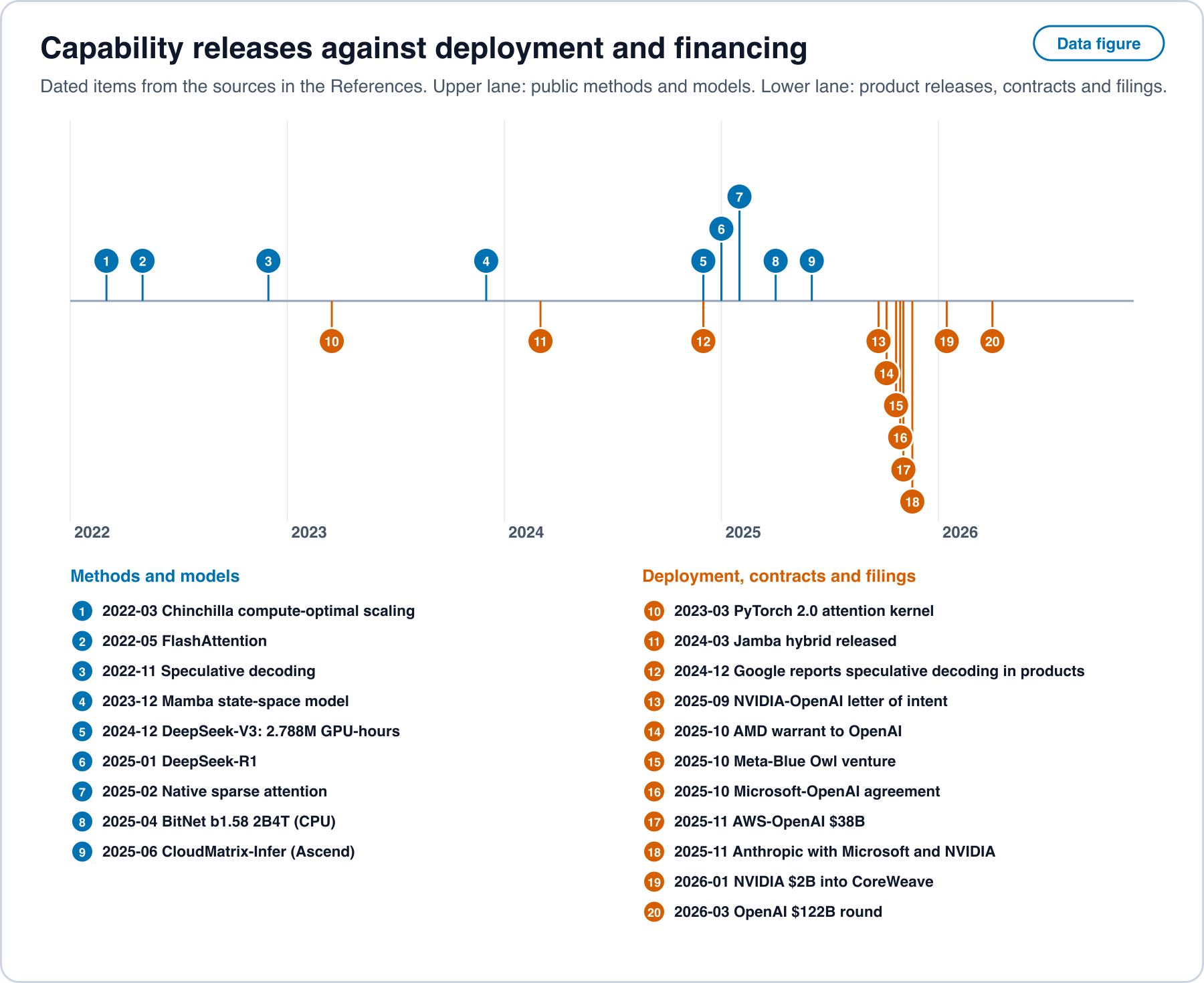
| Architecture | Selective state space models and attention variants are dual through structured semiseparable matrices, and the resulting layer is reported 2 to 8 times faster than the earlier scan [38]. | 31 May 2024 | established by proof in the source |
| Architecture | Hybrid state space and attention models were released with open weights by several groups across 2024 and 2025 [39]. | 2024 to 2025 | demonstrated |
| Number format | Ternary weights match 16-bit perplexity and end-task scores from about 3 billion parameters at lower latency, memory and energy, in the authors’ experiments [40]. | 27 Feb 2024 | demonstrated |
| Number format | Stable 4-bit pretraining of a 12 billion parameter hybrid model on 10 trillion tokens, comparable to 8-bit results, reported by the hardware vendor [41]. | Sep 2025 | demonstrated |
| Kernels | An attention kernel reaches up to 75% of peak 16-bit throughput on one accelerator generation, against 35% for its predecessor [42]. | Jul 2024 | demonstrated |
| Sparsity | Hardware-aligned, natively trainable sparse attention with reported speedups at 64 thousand tokens of context [43]. | Feb 2025 | demonstrated |
| Decoding | Speculative decoding leaves the output distribution unchanged and was measured at 2 to 3 times faster on a large translation model [23]. | 30 Nov 2022 | established by proof in the source |
| Scaling | When lifetime inference demand is counted, the cost-optimal model is smaller and trained on more tokens than the training-only rule gives [44, 45]. | Jan 2024 | demonstrated |
| Training cost | A frontier-scale model reported at 2.788 million accelerator-hours for full training, using latent attention and 8-bit training [46]. | 26 Dec 2024 | demonstrated |
| Conformal inference | Finite-sample, distribution-free coverage for any predictor, with proofs collected in a book [47]; a survey first posted in October 2024 and published in 2025 covers structured, unstructured and dynamic data [48]. | 18 Nov 2024 | established by proof in the source |
| Inference with predictions | Valid intervals from a small labeled set and many machine predictions, for any predictor [49]. | 2023 | established by proof in the source |
| Sequential inference | E-processes and confidence sequences that stay valid when a test is stopped at any time [50]. | Nov 2023 | established by proof in the source |
| Causal estimation | Debiased machine learning gives valid inference on a target parameter with flexible nuisance models, extended to identifiable effects beyond back-door adjustment [51, 52]. | 2018; 2021 | established by proof in the source |
| Compilers | Compiler passes for higher-order automatic differentiation report up to 1.3 times on second-order operators, preliminary [53]; a 2026 methodology paper states that compiled JAX far exceeds Stan’s efficiency on modern hardware, with no benchmark numbers in its abstract [54]. | 2025 | demonstrated |
| Probabilistic programming | A compiler that keeps probabilistic semantics reports a geometric-mean 6.4 times over Stan and 53 times over Turing on standard benchmarks [55]. | 2025 to 2026 | demonstrated |
| Energy measurement | An open benchmark measures inference energy across 40 architectures and reports time and energy Pareto configurations with savings above 40% in some cases [56]; one provider reports 0.24 watt-hours for a median text prompt in production [57]. | 2025 | demonstrated |
Two rates give the background. Compute needed to reach a fixed language-model score has halved about every 8 months, with a 95% interval of about 5 to 14 months [58]. The price of reaching a fixed benchmark level fell between 9 and 900 times a year across six benchmarks, median about 50, with the fastest rates resting on under a year of data [59]. Both are rates of change in the capability frontier or a price, and neither measures the gap to deployment.
Two limits apply to the table. Several rows are speedups against a baseline chosen by the authors, so the numbers do not add or compare across rows. And “possible” in these rows means demonstrated by the authors in a stated setting, not available in a product.
3. What the gap looks like in data
Long-run diffusion. Across 15 technologies and 166 countries from 1820 to 2003, the average lag between invention and adoption in a country was about 45 years, and lags shrank over the period [60]. The same history carries a warning about what adoption means. Electric motors raised factory productivity only after plants were redesigned around one motor per machine, a change that took decades [61]. A later model attributes the dip and rise in measured productivity to unmeasured complementary investment in processes and skills [62]. In both accounts the delay is mostly the cost of reorganizing around the tool, which in the notation above is .
Open release to consumer hardware. For models that fit one consumer graphics card, the average lag behind the best model overall was 6 to 12 months across four measures in 2025, with the largest lag, 12.4 months, on a preference score [63]. A broader analysis of open-weight models of any size found about one year, with a range of 5 to 22 months by benchmark, and a later index-based analysis put the average near 3 months [64]. These figures measure the distance between two public frontiers. They are lower bounds on a lag to products, because an open model on a card is not yet a product anyone is paid to support.
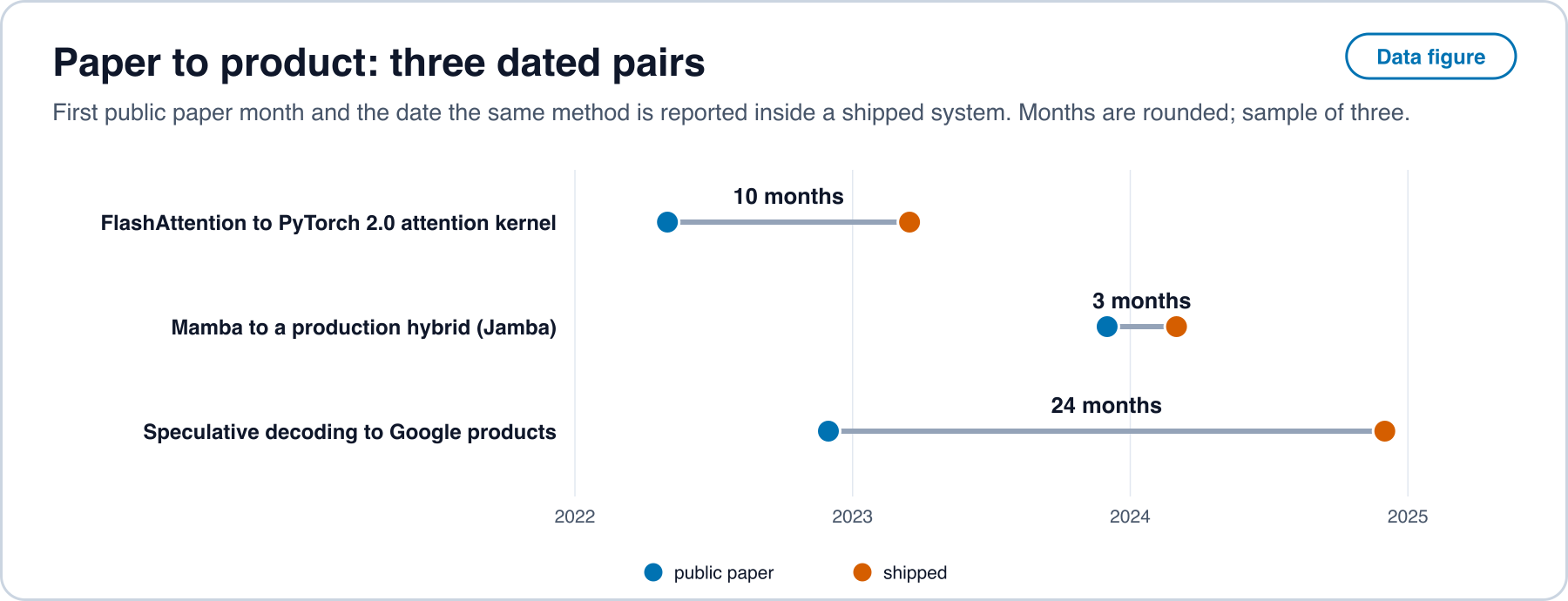
From paper to product. Speculative decoding was posted in November 2022. Its authors’ employer reported applying it in products by December 2024 [24]. A practitioner account from the same month says that production use needed extra work on batching, quality and reliability and helps mostly at limited batch sizes [65]. Two more pairs are in Section 13. A few dated pairs are not a distribution, and the protocol in Section 16 specifies how to collect many. A longer-run measure of the paper-to-patent distance finds that patent citations to articles are on average 14.4 years older than the patent on the front page and 16.6 years when in-text citations are counted [66], and linked patents and papers are typically two to four citation steps apart [67]. Those figures are for science broadly and are not about machine learning in particular.
Practice of 4-bit models. Practitioner accounts date the point at which 4-bit local inference became workable on consumer machines to 2023 [68]. The accounts are narrative, so this is opinion-class evidence for a date and not a measurement.
Firm adoption. The United States Census Bureau’s 2026 supplement found 18% of firms using AI in a business function in November 2025 to January 2026, 22% expecting to within six months, and 57% of users in three or fewer functions [34]. In the European Union, 20.0% of enterprises with 10 or more employees used at least one AI technology in 2025, up 6.5 points from 2024, with 55.0% of large, 30.4% of medium and 17.0% of small enterprises [33]. The OECD reports 13.9% adoption in 2024 and 39% of large firms against 12% of small firms [35]. Chinese hiring data show generative-AI hiring at 21% of listed firms against 0.2% of unlisted ones at the end of 2025 [69]. Survey wording and sampling frames differ by source, and the Census question was revised in November 2025, so rates are not comparable across rows.
Official statistics in the original languages. Germany’s Statistisches Bundesamt reports that 20% of firms with 10 or more employees used AI in 2024, against 12% in 2023 and 11% in 2021, with 48% of large, 28% of medium and 17% of small firms, and names lack of knowledge and legal uncertainty as the most common reasons for not using it [70]. Its 2025 table gives 26% overall and 57% for firms with more than 250 employees, on a changed enterprise definition [31]. Insee reports 10% of firms in France using AI in 2024, four points above 2023, 33% of firms with 250 or more employees, and 42% in information and communication against 5% or less in transport, accommodation and food, and construction [37]. Spain’s Instituto Nacional de Estadística reports 21.1% of firms with 10 or more employees using AI in the first quarter of 2025, 8.7 points higher than a year earlier [32]. Brazil’s Cetic.br reports 13% of firms using AI in 2024, the same share as in 2023, concentrated in large firms and in information and communication [36]. Korean ministry statistics, as reported in the Korean press, give 32.9% of firms using AI technology or services in 2024 against 30.3% in 2023, and 66.9% for firms with 250 or more workers [30]. Japan’s white paper surveyed workers in four countries and found any business use of generative AI at 55.2% in Japan, 90.6% in the United States, 90.3% in Germany and 95.8% in China. Among Japanese firms, 49.7% had an active or limited-use policy in 2024 against 42.7% a year earlier, and the most common Japanese concern, at 30.1%, was not knowing how to use it effectively, against 9.7% in the United States and 10.4% in China [71]. China’s CNNIC counts 515 million generative-AI users in June 2025, 266 million more than in December 2024, a penetration of 36.5% [72]. These are measurements of use, not of release. Within each country the rate rises with firm size, which is consistent with a fixed adoption cost weighing less on a large budget, though the surveys cannot separate that from other causes.
Use at the level of people and tasks. Nearly 40% of United States adults aged 18 to 64 used generative AI in late 2024, and about 23% of workers had used it at work in the prior week [73]. A field study of 5,179 customer-support agents found 14% more resolutions per hour on average and 34% more for novice and low-skilled workers [74]. A randomized trial with 16 experienced developers and 246 tasks found tasks with AI allowed took 19% longer in that setting [75]. These results differ because tasks, people and tools differ. They show that deployment is not a single event, which is why is defined from offers and not from use.
What slows research itself. Research effort has risen while research productivity has fallen in most sectors, and keeping chip density doubling needed more than 18 times the researchers of the early 1970s [76]. This bears on , not on , and is noted so the article does not read the capability frontier as free.
4. Calendars: reporting and funding periods
Decision dates in listed firms follow the reporting calendar. In a survey of 401 financial executives, 78% would give up economic value to smooth reported earnings, and 55% would avoid starting a very positive net-present-value project if it meant missing the quarter’s consensus [77]. Comparable public firms invest less, and respond less to investment opportunities, than private firms [78]. All of these are demonstrated for earlier technologies and periods, and none is a measurement of AI releases.
Attention follows the same calendar. The count of United States large-company earnings calls citing “AI” reached 306 in the third quarter of 2025, against a ten-year average of 86 [79]. Earnings-call language has been used as a measurement instrument for other topics, validated against manual reading [80], and the same instrument can be pointed at release topics.
Funding follows a longer calendar. A venture fund has a finite life, typically ten years, and firms raise new funds every three to five years [81]. Partnership agreements specify finite lifetimes, usually ten years [82]. The two calendars differ in length, about a quarter and three to five years, and both quantize when a commitment can be made. Proposition 1 below uses only that structure.
5. Control and incumbent response
Two older results frame the incentive to deploy. Arrow’s analysis finds the incentive to invent smaller under monopoly, meaning barriers to entry, than under competition, and counts a temporary monopoly that does not bar entry as nearly competitive [83]. A later review of the competition and innovation literature notes that preemption incentives are a force missing from simple static models [84]. Incumbents also miss changes that rearrange known components, because their routines filter what they notice [85]. Neither is a statement about any firm now.
Control over distribution is documented in public court records. In September 2025 a United States district court barred exclusive distribution contracts for several search and assistant products, allowed non-exclusive default payments with terms generally limited to one year, and ordered data sharing and syndication remedies [86]. The article uses the record only as evidence that defaults and distribution terms are priced and regulated, which is what the parameter in Section 6 represents.
6. The model
Setting. One buyer population with demand per period for a task at price . An incumbent serves it at cost with an existing method. A public method becomes available to anyone at cost , non-increasing in time. A buyer can switch to a seller using the public method at friction per task, so the incumbent’s price ceiling is . The incumbent may release an offering built on the public method at one-time cost . Decisions are made only at dates .
Assumptions.
- A1. Linear demand , with .
- A2. The public cost declines: is non-increasing and continuous with , and .
- A3. The ceiling binds on the incumbent’s price, that is for the cost it faces. This holds for the numbers in Section 7.
- A4. The incumbent maximizes discounted profit at rate subject to a reporting rule: a share of is expensed in the release period, and the release period’s reported earnings must not fall short of the pre-release level by more than .
- A5. After release the incumbent’s cost is , the cost of the public method.
- A6. Flow gains from release are treated as constant after the release date (steady-state approximation).
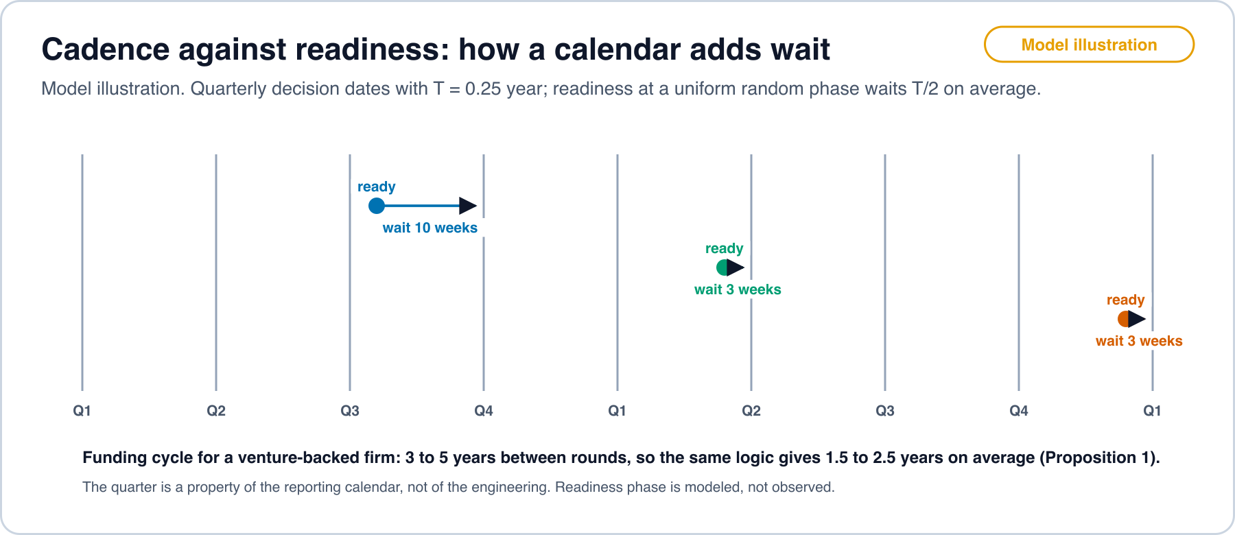
Proposition 1 (calendar quantization). If a method becomes ready at time and the firm releases at the first decision date at or after when release is worthwhile, the wait is . If is uniform on , then and .
Derivation. Write with uniform on . For the next date is and the wait is , which is uniform on . A uniform variable on an interval of length has mean and variance . The case has probability zero.
Consequence. A firm deciding on a quarterly calendar adds on average about 6 weeks, and one deciding on a funding cycle of 3 to 5 years adds 1.5 to 2.5 years, to the readiness delay , with no engineering cause. The assumption that readiness is uniform within a period is the weak part, and Prediction 1 tests the converse.
Proposition 2 (release threshold and forced release). Define the flow gain for the outside cost . On , is strictly decreasing in . Without calendar or reporting constraints, release is optimal exactly when , that is when , where is the unique solution of if it exists. If , holding earns no profit, and release is preferred to holding. A reporting rule can delay it but cannot make holding profitable.
Derivation. Under A3 the incumbent holding at cost prices at the ceiling, so its profit is . After release its cost is and its profit is . The difference is . Differentiating, on the stated range, so is strictly decreasing. With A6 the value of release is , which is non-negative exactly when . Holding yields profit , which is zero at , that is at , and negative below. Release at that point yields profit by A1.
Proposition 3 (reporting gate, delay and a never-release region). Under A4 the release-period reported earnings change is . Release is allowed if this is at least , that is if . Define and . Then , the release date moves from to or to the forced-release point , whichever is earlier, and for the delay is when . If , where is the cost floor, release never occurs on the NPV and gate conditions, and only the forced release at applies if .
Derivation. Reported earnings in the release period gain of operating profit and lose the expensed part of the adoption cost. Requiring the net to be at least gives the stated inequality. Since is strictly decreasing (Proposition 2), the larger of two required gains corresponds to the smaller cost threshold, so . With the time to reach is , and the difference of two such times is the stated delay. The attainable gain is at most because by A2.
Proposition 4 (forcing function). Suppose an automation tool lowers the adoption cost from to . (a) The NPV threshold rises, so release is optimal earlier. (b) If , the reporting gate does not bind, , and . (c) The total latency of the firm falls to , where is the technical readiness delay with the tool.
Derivation. (a) and is strictly decreasing, so lowering lowers the required gain and raises . (b) The gate condition is satisfied by every when the right side is non-positive, which is . Then . (c) Follows from Definition 2 and Proposition 3.
Reading. A tool acts as a forcing function in two separate ways. It lowers and so removes the gate delay once passes under . And it lowers for every seller, which forces release at , where holding earns nothing. The first is a property of the adopting firm and the second a property of the market.
Proposition 5 (market latency is set by the least constrained firm). If over firms that can sell to the buyer population, then .
Derivation. , and does not depend on . Subtracting gives the result.
Consequence. A calendar or gate that delays one firm does not delay the market when another firm can reach the same buyers without that delay. The latency observed in a market is then the latency of the fastest firm that has access. Where access is restricted, because buyers cannot reach other sellers, the minimum is taken over a smaller set. In the model this is the role of .
Proposition 6 (what remains to charge for). After release, with the ceiling binding, price is , profit is , and the margin per task is , independent of . Price changes one-for-one with cost, while the price to cost ratio rises as cost falls. The marginal value of friction is , which is positive for and increases as falls.
Derivation. Under A3 the incumbent charges the ceiling . With cost , the margin is and volume is , giving . The ratio follows from . Differentiating in gives , and .
Reading. As the cost of computing falls, the part of price that reflects computing shrinks, and the remaining margin depends on how costly it is for a buyer to leave. Spending that raises becomes worth more. In the model this is a statement about incentives and not a judgment of any firm. Policies that lower , such as limits on default terms or portable data formats, lower the margin by the same amount, and the model does not say whether that is desirable.
7. A numerical illustration, not a fit
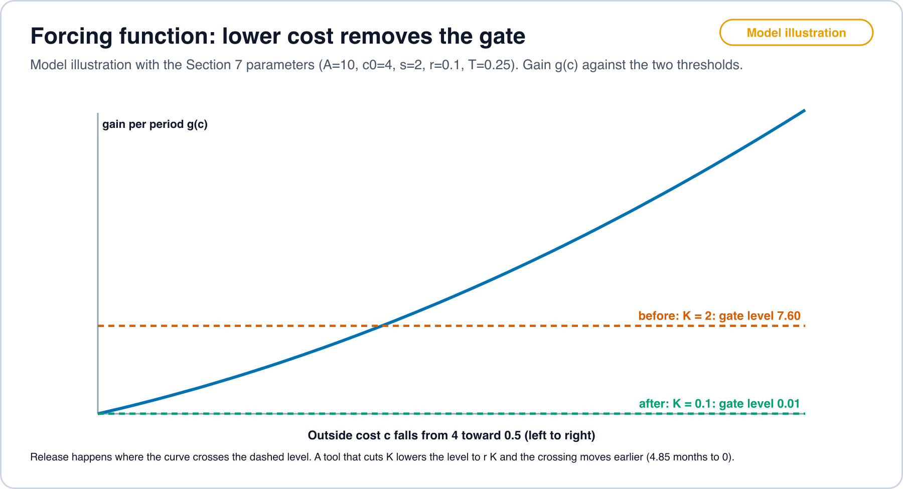
The script model_check.py in the work folder reproduces these numbers with the standard library. Parameters: , , , per year, year, , , and outside cost halving every 8 months so . The 8-month rate echoes [58] and is a choice for illustration, not an estimate for cost.
Table 2. Release date with and without an adoption-cost-lowering tool.
| Case | NPV threshold | Gate threshold | Release at | Gate delay | |
|---|---|---|---|---|---|
| Before the tool | 2.0 | , day 4 | month 5.00 | 4.85 months | |
| Tool lowers adoption cost | 0.1 | day 0.2 | 0 |
In the first row the gate requires a gain of , far above the NPV requirement , so the incentive-delay part is 4.85 months. That is longer than the calendar term of Proposition 1 for a quarterly firm, which is 1.5 months on average. In the second row , so the gate does not bind and only the NPV condition remains, as in Proposition 4(b).
model_check.py and Table 2. Open full sizeTable 3. After release, with .
| Price | Profit | |||
|---|---|---|---|---|
| 4.0 | 6.00 | 1.50 | 8.00 | 2.00 |
| 3.0 | 5.00 | 1.67 | 10.00 | 3.00 |
| 2.0 | 4.00 | 2.00 | 12.00 | 4.00 |
| 1.0 | 3.00 | 3.00 | 14.00 | 5.00 |
| 0.5 | 2.50 | 5.00 | 15.00 | 5.50 |
Profit rises as cost falls because linear demand lets volume expand. With satiated demand the profit column would flatten, and the claim about margin staying at would not change. A simulation of Proposition 1 with and uniform readiness gives a mean wait of 0.1250 against and variance 0.00521 against (200,000 draws, seed 7).
8. Predictions and what would refute them
Each prediction names the data, the test and the result that would count against the model. Predictions are stated before any of the data was collected.
Prediction 1 (calendar clustering). The dates on which firms with quarterly reporting make previously open methods generally available are not uniform within the quarter. Test: for a sample of at least 200 releases from listed firms, compute each date’s phase within the firm’s fiscal quarter and apply Rayleigh and Kuiper tests against uniformity. Refuted if the null of uniform phase is not rejected at 5% with 200 or more independent items.
Prediction 2 (listed against unlisted). For the same method and comparable difficulty, the median delay from open release to a generally available product is longer for listed firms than for firms funded outside a reporting calendar. Test: matched pairs by method, with firm type as the treatment and hazard ratios for time to release. Refuted if the 95% interval of the hazard ratio (listed over unlisted) lies entirely above 0.8.
Prediction 3 (tools lower the gate). After an automation tool that lowers porting cost becomes available for a hardware or software target, time from open release to general availability on that target falls. Test: difference in differences with targets served and not served by the tool, with release delay in days as outcome. Refuted if the 95% interval of the estimated change lies entirely above days. The 30-day margin is a protocol choice made before data collection.
Prediction 4 (price outruns cost). Where joule and hardware costs per task are measured, the ratio of list price to cost per task rises as measured cost falls. Test: panel of services with a stated task, using open energy measurements and list prices. Refuted if the ratio is flat or falls in more than half of tasks over a period in which cost fell by a factor of 2 or more.
Prediction 5 (spending moves to friction). In a market where cost per task falls, the share of seller revenue spent on distribution, defaults and bundling rises. Test: disclosed distribution payments and bundling terms in filings and court records against revenue. Refuted if the share is flat or falls while cost per task falls by a factor of 2 or more.
Prediction 6 (market latency follows the fastest firm). In markets where buyers can reach more than one seller at low friction, market latency is close to the minimum firm latency, and in markets with high measured friction it is closer to the median. Test: regress market latency on measured switching friction. Refuted if the 95% interval of the slope on friction lies entirely at or below zero.
Predictions on the financing and cost of the build-out. The predictions in Sections 10 and 12 concern the money flows and the cost of an accelerator-hour. They are stated in those sections, and they are tested on filings and listings dated after this article.
What would refute the model itself. A finding that release dates are uniform within the quarter for listed firms (Prediction 1), that listed and unlisted firms release at the same pace (Prediction 2) and that porting-tool arrival does not change delay (Prediction 3) would leave no role for calendars or reporting gates, and the artificial latency of Definition 2 would be zero in measurement. The model would then reduce to engineering delay .
9. The money loop: what the filings document
A common description of the current build-out is a circular economy: labs buy compute from clouds, clouds and neoclouds buy chips and memory, and chip makers and clouds invest in the labs. This section sets out what dated documents say about that description. It gives no verdict. Each item is marked documented when a filing, a dated release or an official statistic states the amount and the counterparties, inferred when it follows by arithmetic from documented figures under a stated assumption, and not found when the sources read do not say.
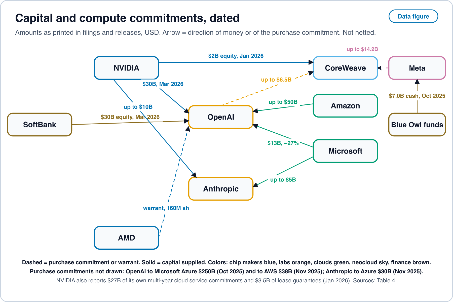
scripts/figures/latency_figures.py with latency_data/flows.csv; sources are listed in Table 4. Open full sizeCapital supplied to customers. In the round of 122 billion dollars that OpenAI closed in March 2026, NVIDIA is reported at 30 billion dollars, Amazon at up to 50 billion and SoftBank at 30 billion [9]. An earlier letter of intent had said NVIDIA intended to invest up to 100 billion dollars progressively as each gigawatt is deployed, which is a statement of intent and not a closed transaction [87]. Microsoft reports about 27% of the OpenAI public benefit corporation and 13 billion dollars of total funding commitments accounted under the equity method [7]. For Anthropic, NVIDIA and Microsoft committed to invest up to 10 and 5 billion dollars [10]. NVIDIA bought 2 billion dollars of CoreWeave Class A stock after the end of that company’s 2025 fiscal year [4]. AMD issued OpenAI a warrant for up to 160 million shares at 0.01 dollars per share, vesting in tranches tied to purchases of AMD Instinct GPU products [88].
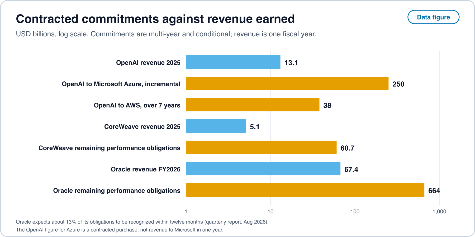
Purchases committed by customers. OpenAI contracted to buy an incremental 250 billion dollars of Azure services [7, 89], a 38 billion dollar agreement with AWS that the announcement describes as growing over seven years [8], and up to 6.5 billion dollars from CoreWeave, while Meta has an order form with CoreWeave of up to 14.2 billion [4]. Anthropic committed to buy 30 billion dollars of Azure compute and to contract up to one gigawatt more [10]. NVIDIA itself reports 27 billion dollars of multi-year cloud service commitments and 3.5 billion dollars of land, power and shell guarantees to early-stage partners [3].
Table 4. What is documented, what is inferred, and what the sources do not say.
| Item | Documented | Inferred, with the assumption | Not found in the sources read |
|---|---|---|---|
| Equity from suppliers into customers | The amounts and dates above [9, 10, 4] | None drawn | Whether any equity is conditioned on purchases, except the AMD warrant, whose vesting is tied to GPU purchases in the filing [88] |
| Purchases by labs from clouds | Azure 250 and AWS 38 billion dollars for OpenAI; Azure 30 billion for Anthropic [7, 8, 10] | the AWS figure averages about 5.4 billion dollars a year if spread evenly over seven years | The term and ramp of the Azure commitment; the conditions attached to the 50 billion dollar Amazon figure |
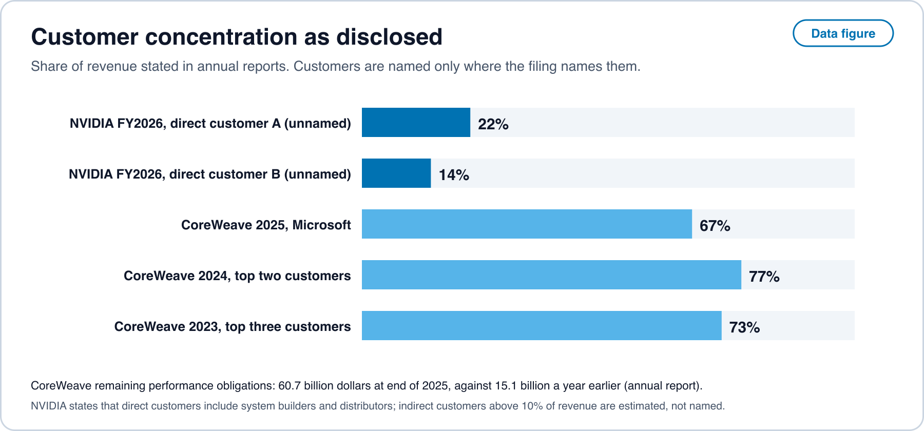
| Customer concentration | NVIDIA direct customers at 22% and 14% of revenue, with system builders and distributors among direct customers [3]; CoreWeave with Microsoft at 67% of 2025 revenue [4] | A lower bound on the Herfindahl index from the disclosed shares: at least 0.068 for NVIDIA and 0.449 for CoreWeave | Who stands behind NVIDIA’s direct customers |
| Customer prepayments | Oracle’s deferred revenue from customer prepayments with a significant financing component rose by 11.4 billion dollars in the quarter, inside operating cash flow of 23.1 billion [5] | About half of that quarter’s operating cash flow came from prepayments | Which customers prepaid |
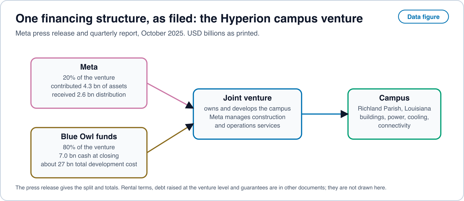
| Venture-level financing | Blue Owl funds hold 80% and Meta 20% of a venture for the Hyperion campus; the funds contributed 7.0 billion dollars cash against about 27 billion dollars of development cost [2, 1] | The cash is about a quarter of development cost | Lease terms, debt raised by the venture and guarantees |
| Depreciation lives | Stated lives for servers in Figure 12 [4, 14, 15, 16, 17] | Moving a life from 5 to 6 years lowers the straight-line annual charge on the same assets by one sixth | The service life that GPUs reach in use |
| Cash capital against operating cash | The annual series in Figure 8 [11] | The ratio of the two | Finance leases and off-balance-sheet leases |
The term customer in this table follows each filing’s own use. Money is fungible, so a filing can show that capital went to a customer and that the customer paid the supplier, and it cannot show that the one funded the other. Section 10 states a test that works within that limit.
Concentration and backlog. Disclosed customer shares are high at the leveraged nodes and lower at the largest chip maker. CoreWeave reports its top three customers at 73% of 2023 revenue, its top two at 77% in 2024 and Microsoft alone at 67% in 2025 [4]. Its remaining performance obligations of 60.7 billion dollars are 11.8 times its 2025 revenue of 5.131 billion. Oracle reports obligations of 664 billion dollars at 31 August 2026 and expects about 13% of them to be recognized in the next twelve months [5, 6], against fiscal 2026 revenue of 67.4 billion [11]. OpenAI reported revenue of 13.1 billion dollars for 2025 and stated a rate of 2 billion dollars a month in March 2026 [9]. Contracted purchases are multi-year and conditional on terms that these figures do not show, so they are not revenue in one year and are not additive with the figures above.
Labs are also buying elsewhere. Anthropic announced a plan to use up to one million TPUs, worth tens of billions of dollars and well over a gigawatt of capacity in 2026 [90]. OpenAI announced a plan to deploy 10 gigawatts of accelerators of its own design [91] and holds the AMD warrant above. A lab that buys from several suppliers and designs its own parts is not a single customer of any one of them, which matters for the bound in the next section.
10. A closed-loop test and its predictions
The question the documents cannot answer by themselves is how much of a supplier’s revenue is paid for with money the supplier supplied. The test below turns it into quantities that a filing can bound.
For a window (a fiscal year), let be capital supplied by supplier to customer (equity, loans, guarantees, warrants valued at issue), let be the revenue receives from , let be the total revenue of , and let be the capital raises from all sources.
Definition 3 (round-trip ratio). , capital supplied per dollar of revenue received from the same counterparty.
Definition 4 (closed-loop share bound). . A customer cannot have paid with more of ‘s own capital than supplied, nor than it paid, so is an upper bound on the share of that could have been funded by ‘s own capital. The customer-side counterpart is , the share of capital raised by that came from its own suppliers. Both are bounds computed from disclosed figures. They are not estimates of what happened, because money is fungible.
Proposition 7 (when a supplier-financed purchase pays). Let supplier sell at price with unit cost and gross margin . Let it supply capital that induces a share of sales that would not otherwise occur, and let it recover value from its stake. The incremental profit is . If all of is spent with , so that , then if and only if , where .
Derivation. Substitute and solve . (By hand, not machine-checked.)
Consequence. Since , supplier financing pays through induced sales alone only when . With the gross margin of 71.1% reported by NVIDIA for fiscal 2026 [3], the stake must be expected to recover at least 28.9% of the capital. Model output for the breakeven induced share at recovery 0, 25%, 50%, 75% and 100% is 1.41, 1.05, 0.70, 0.35 and 0, so with no recovery no share of induced sales is enough.
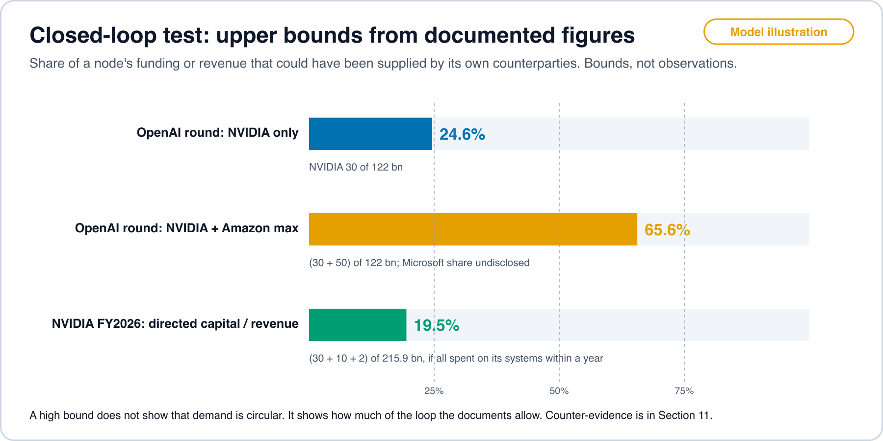
latency_data/model_outputs.json, computed by model_airace.py from [9, 10, 4, 3]. Open full sizeBounds from the documents. NVIDIA’s share of the OpenAI round is at most 24.6%, and with Amazon at its stated maximum the two reach at most 65.6%, with Microsoft’s part not disclosed (model output). Capital that NVIDIA announced or was reported to supply to customers from November 2025 to March 2026 is 42 billion dollars (30 for OpenAI, up to 10 for Anthropic and 2 for CoreWeave), which is 19.5% of its fiscal 2026 revenue of 215.9 billion and 41% of its operating cash flow of 102.7 billion [3, 11]. The first figure is a scale comparison, since the amounts and the revenue year differ. Read as a bound, it means that if every one of those dollars came back as NVIDIA revenue within one year, at most about a fifth of that year’s revenue would be funded by NVIDIA’s own capital.
Predictions. Each names data, a test and a result that would count against the claim. These predictions were written after the filings above were read, and they are tested on filings dated after this article.
Prediction 7 (the loop share stays bounded). For each chip or cloud supplier with disclosed directed capital, computed from each annual report stays below 0.25 while revenue from customers that received no directed capital grows at least as fast as revenue from those that did. Test: annual filings, with customers named where filings name them. Refuted if exceeds 0.5 in a fiscal year, or if revenue growth is concentrated in customers that received directed capital. Values between 0.25 and 0.5 are inconclusive.
Prediction 8 (end-user revenue outgrows commitments). For a lab, the ratio of contracted purchases to trailing twelve-month revenue falls over four consecutive quarters while revenue rises. Test: lab statements and cloud backlog disclosures. Refuted if the ratio rises for four consecutive quarters.
Prediction 9 (stress shows first where concentration and leverage are highest). When a lab revises a compute commitment downward, the size of revisions to guidance at supplier nodes is ordered by their disclosed top-customer share. Test: guidance revisions after any such event, ordered by disclosed top-customer share. Refuted if the order is unrelated to concentration.
Prediction 10 (substitution reduces committed capacity per dollar of revenue). Where open methods and cheaper hardware reduce accelerator time per task (Section 12), committed gigawatts per dollar of lab revenue fall. Test: announced capacity and lab revenue by quarter. Refuted if committed gigawatts per dollar of revenue rise for four consecutive quarters while measured accelerator time per task also falls on open benchmarks.
11. The strongest counter-evidence
The reading that the build-out is mostly a closed loop meets four sets of documents that point the other way, and one set that points toward fragility.
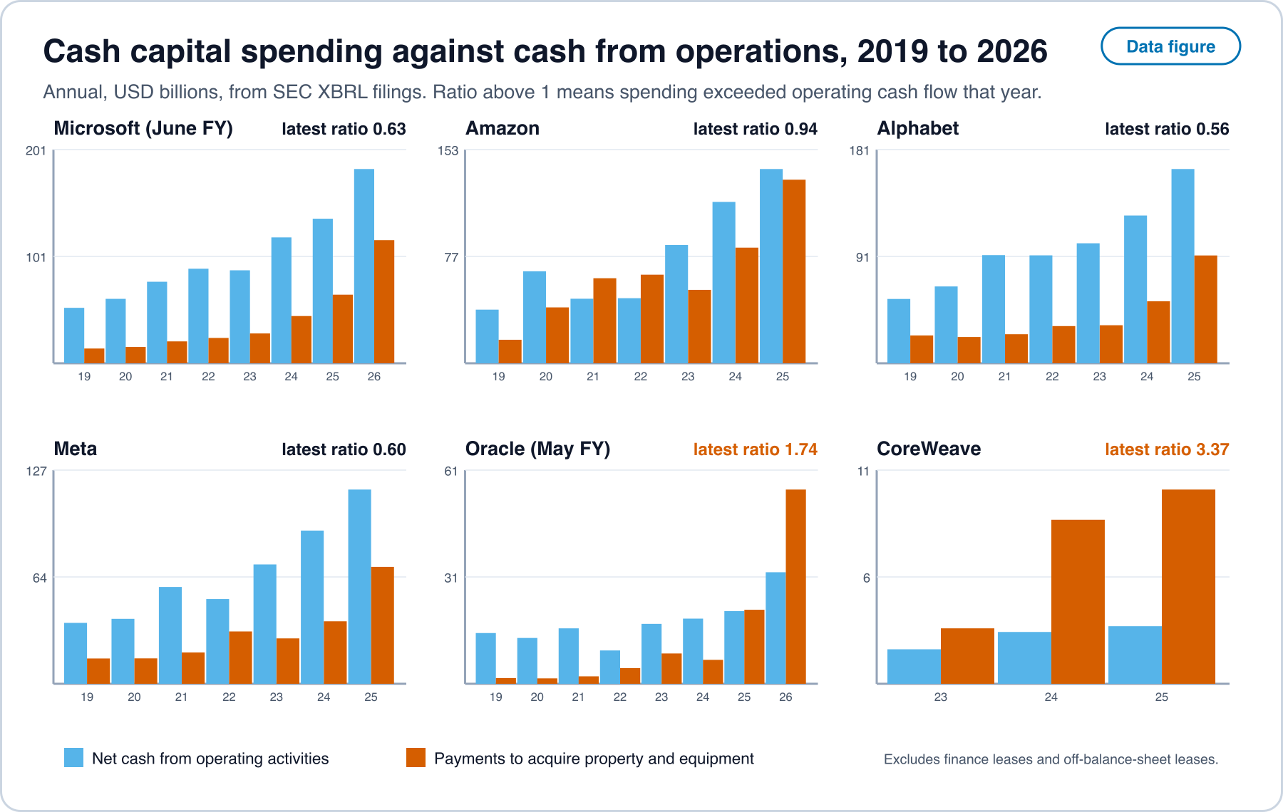
Most spending is funded from operations at the largest buyers. In their latest fiscal years, cash capital spending was 0.63 of operating cash flow at Microsoft, 0.94 at Amazon, 0.56 at Alphabet and 0.60 at Meta [11]. The spending is large, and it is paid for out of cash that the same firms earn from other businesses.
latency_data/capex_ocf.csv [11]. Open full sizeThe largest chip supplier could fund its directed capital from its own cash. The 42 billion dollars above is 41% of one year’s operating cash flow at NVIDIA [3, 11], and its two largest direct customers are 22% and 14% of revenue, with system builders and distributors among them [3].
Revenue from end users is real and growing in the statements read. OpenAI reported 13.1 billion dollars of revenue for 2025 and a rate of 2 billion dollars a month in March 2026, which annualizes to 24 billion (arithmetic) [9].
Labs diversify. Anthropic’s plan for up to one million TPUs alongside its Azure and NVIDIA commitments, and OpenAI’s plans for its own accelerators and the AMD warrant, mean that the labs named here have more than one chip source in their announced plans [90, 10, 91, 88].
What the counter-evidence does not remove. Cash capital spending was 1.74 times operating cash flow at Oracle in fiscal 2026 and 3.37 times at CoreWeave in 2025 [11]. Oracle’s quarter ended 31 August 2026 shows operating cash flow of 23.1 billion dollars with 11.4 billion of that from customer prepayments, and free cash flow of negative 5 billion [5, 6]. CoreWeave’s obligations are 11.8 times its revenue, and its customer base is concentrated [4]. These are the nodes where a shortfall in a lab’s funding would arrive first, which is what Prediction 9 tests.
Net reading, as far as the documents go. Loops of tens of billions of dollars are documented between named suppliers and customers. The documents bound the share of the largest chip supplier’s revenue that its own capital could have funded under a fifth, and show most hyperscaler spending paid from operating cash. The concentrated and leveraged nodes, a cloud with prepayments and a neocloud with a single dominant customer, are where the loop assumption would matter most. Terms of private agreements are not public, so the documents give bounds and not a measurement.
12. What a task costs: the infrastructure cost model
Section 0 defines cost per task as . This section fills in and from the cost of an accelerator-hour and ties the result to , and .
Accelerator-hour. Let be capital per accelerator, including the share of facility, power and cooling, with straight-line life years and utilization . Capital per utilized hour is . Let be facility power per accelerator in kilowatts and the price of electricity per kilowatt-hour. A task that occupies utilized hours costs
Proposition 8 (the capital-loaded price of a joule). At fixed hardware, with per kilowatt-hour equivalent, so joules per task stays the right unit of account, and the price that converts joules into dollars is dominated by whenever . Derivation. Eliminate between the two expressions. (By hand.)
Inputs. The Epoch AI data-center dataset gives, for 74 sites with both figures, median capital of about 33,300 dollars and 880 watts of facility power per H100-equivalent, with capital per H100-equivalent ranging from about 19,600 to about 200,800 dollars [12]. These are estimates built from public permits and imagery, and a site’s listed capital includes compute, construction and fit-out.
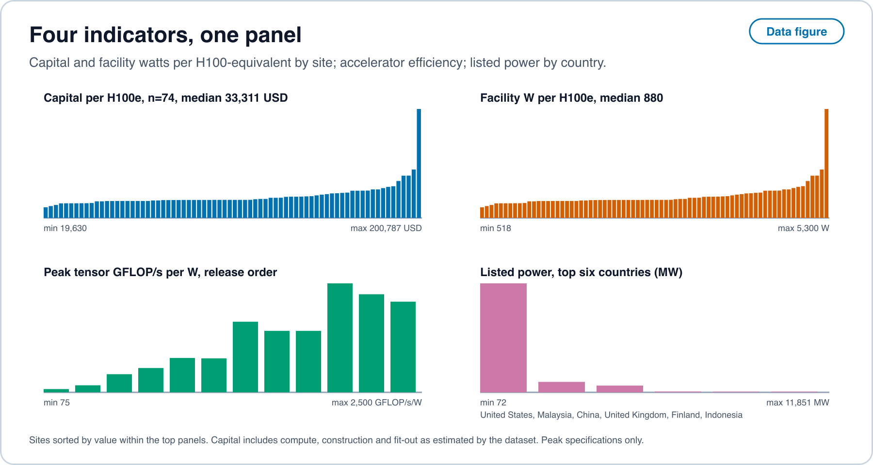
latency_data/frontier_dc_cost_per_h100e.csv, hardware_flops_per_watt.csv, frontier_dc_by_country.csv [12, 13]. Open full sizeModel output. With lives of 4 to 6 years, utilization of 40% to 80% and electricity at 0.04 to 0.12 dollars per kilowatt-hour, an utilized accelerator-hour costs between about 0.83 and 2.5 dollars, and energy is between 1.5% and 11.8% of it. The capital-loaded price is about 0.9 to 2.7 dollars per kilowatt-hour equivalent, against electricity at 0.04 to 0.12, so is dominated by capital at roughly 8 to 70 times the electricity term.
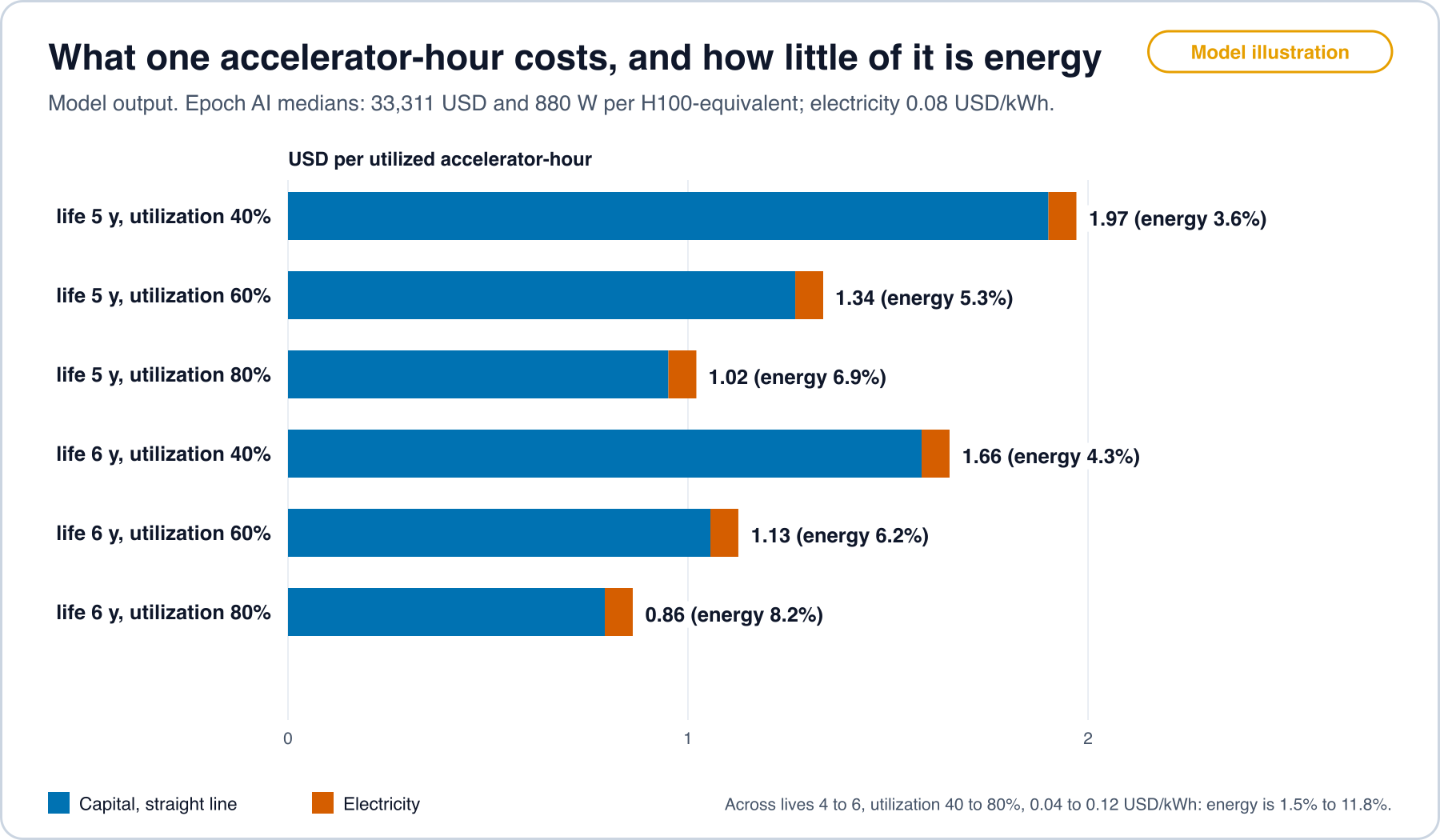
latency_data/model_outputs.json, computed by model_airace.py from [12]. Open full sizeThree consequences follow. Cheaper electricity can lower the cost of a task by at most the energy share, which is at most about an eighth in this grid. Utilization matters as much as energy: halving doubles . And the stated life is an accounting choice that moves in proportion to .
Lives and efficiency. Peak tensor operations per watt rose about 1.42 times a year across twelve leading accelerators from 2016 to 2024 in the vendors’ own specifications, which is a doubling about every two years [13]. A power-limited site that replaced a part with one three years newer would obtain about times the peak operations from the same power. Peak specifications are not delivered energy per task, because utilization, memory traffic and software decide the delivered figure. Stated server lives in Figure 12 run from 5 to 6 years at several large firms, and the range stated is wider at others. Lives of that length and a two-year efficiency doubling are consistent when older parts keep earning at prices set by newer ones, which is a claim about prices and not about physics.
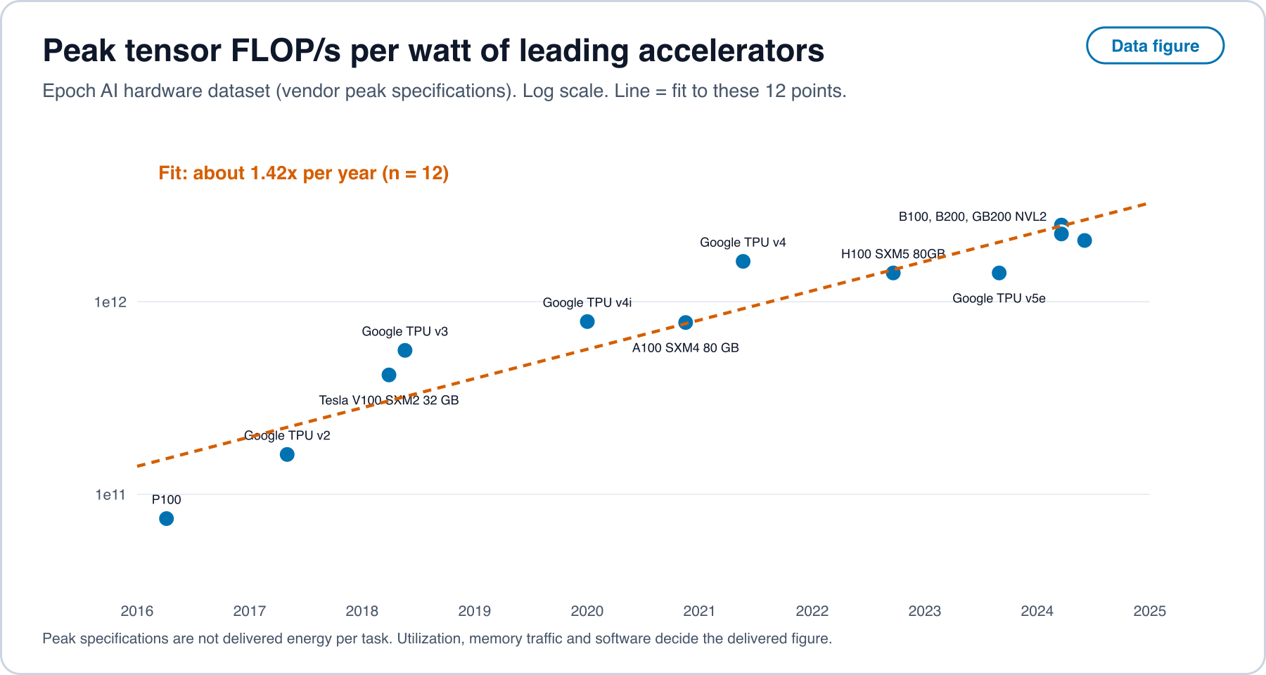
latency_data/hardware_flops_per_watt.csv and hardware_fit.json [13]. Open full size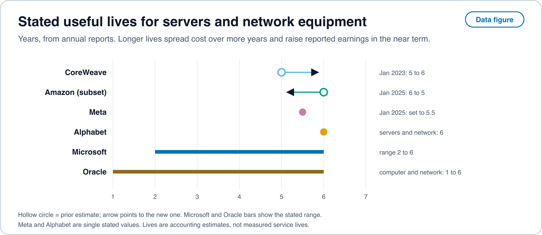
Price is not cost. For a system at the level of GPT-3.5, the price of inference fell more than 280-fold between November 2022 and October 2024, while hardware costs fell 30% a year and hardware energy efficiency improved 40% a year [18]. Over the 1.9 years in that window those rates give about 2.0 times for hardware cost and 1.9 times for energy efficiency (model output). Dividing 280 by 2.0 leaves a factor of about 141 that hardware cost does not explain. That remainder mixes smaller models, algorithmic efficiency, utilization and margins, and the sources do not apportion it. Epoch AI separately estimates that the compute needed for a fixed language-model performance halves about every 8 months [58], and that the price for a fixed benchmark level fell 9 to 900 times a year with a median near 50, the fastest rates resting on under a year of data [59].
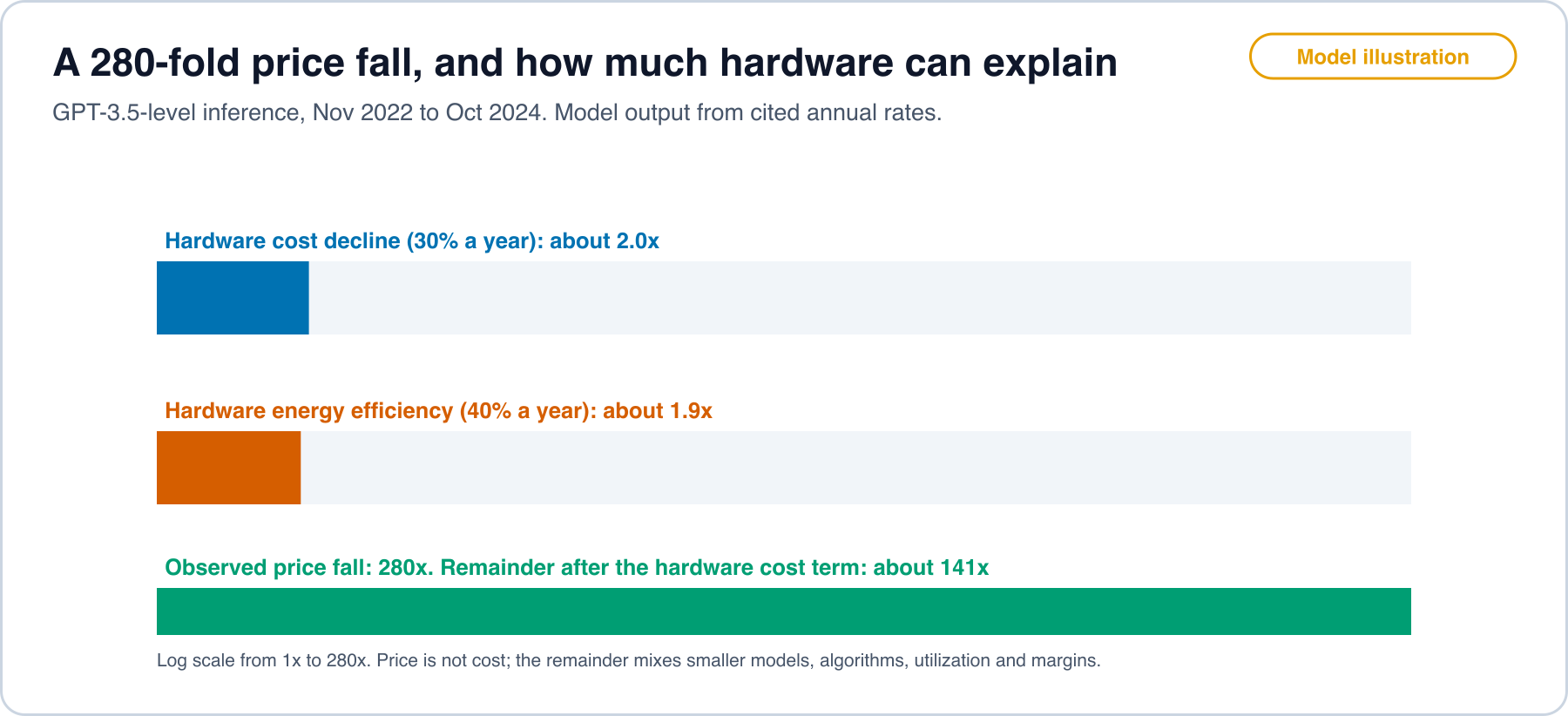
latency_data/model_outputs.json. Open full sizeTie to the frontiers. Let be the lowest accelerator time per task at quality among documented methods and the time in generally available products. Then for the capability frontier, and the deployed frontier follows the price offered, which is at least cost plus the margin of Section 6. Hardware cost enters and in the same way, because suppliers and buyers purchase from the same market, so it shifts both frontiers together and leaves nearly unchanged. Latency is moved by the software term : a method that cuts accelerator time per task by a factor lowers by that factor when it is published, and only when a product adopts it. During the wait, the ratio of the deployed to the capability cost is .
Tie to the cadence model. Capital is committed in multi-year steps and charged over lives of several years, so the decision dates for hardware are far apart, and the adoption cost of Section 6 includes the value of installed capital that a new method would strand or would save. A method that runs on hardware a firm already owns has an adoption cost that is mostly engineering. A method that needs new hardware carries the capital cycle with it. That is why open software methods on existing parts are the least gated, and why Prediction 3 compares targets with and without porting tools.
Where cost stops tracking capability. At a fixed quality , cost per task falls with , with hardware and with price. At the frontier of capability, cost per task is set by the training and serving of the largest models and does not fall in the same way, which is why a frontier-quality task and a fixed-quality task have different cost curves. The data above measure only the first.
Prediction 11 (older parts keep earning). If stated server lives are economically realistic, rental prices per accelerator-hour for parts several years old fall more slowly than peak operations per watt would imply. Test: dated open price listings by part and age, against the efficiency fit in Figure 11. Refuted if the price of an older part per unit of peak operations falls at least as fast as the efficiency fit.
Prediction 12 (energy share stays small). In a sample of measured deployments the energy share of cost per task stays below 15% at electricity prices under 0.12 dollars per kilowatt-hour. Test: open energy measurement of inference [56] combined with listed accelerator-hour prices. Refuted if the measured share exceeds 15% in a majority of deployments.
13. Open methods and existing hardware at parity
A second description of the present is that open algorithmic work lets existing and older infrastructure perform at parity with the newest. The dated record supports a narrower statement, set out here by the lever each method pulls and by the lag to a shipped use.
Table 6. Open methods, their dated papers and what a later use shows.
| Lever | Open method and what the authors report | Posted | Later use | Lag |
|---|---|---|---|---|
| Quantization | Models with 175 billion parameters quantized in about four GPU hours to 3 or 4 bits per weight with negligible accuracy loss [92] | Oct 2022 | 4-bit local inference reported as practical on consumer machines in 2023 [68] | Not computed: the later use is a different 4-bit implementation, and its date is opinion-class evidence |
| Ternary weights on CPU | A 2 billion parameter model at 0.4 GB of non-embedding memory and 29 ms per token on a CPU, against 1.4 to 4.8 GB and 41 to 124 ms for six open full-precision models of similar size [26] | Apr 2025 | Model weights released with the paper | 0 months |
| Attention kernels | Exact attention made faster by accounting for reads and writes between memory levels [19] | May 2022 | Accelerated attention kernels in the PyTorch 2.0 release [20] | About 10 months |
| Serving memory | Paged key-value memory in an open serving system, with higher throughput than prior systems at the same latency [93] | Sep 2023 | Source code released with the paper | 0 months |
| State-space and hybrid models | An attention-free model reporting 5 times the inference throughput of Transformers [21]; a hybrid that fits one 80 GB GPU, with open weights [22] | Dec 2023 | The hybrid, Mar 2024; more hybrids in 2024 and 2025 [39] | About 3 to 4 months |
| Speculative decoding | Output distribution unchanged with 2 to 3 times faster decoding [23] | Nov 2022 | Reported in Google products by Dec 2024 [24] | About 24 months |
| Training cost | 2.788 million H800 GPU-hours for full training, self-reported [46]; reasoning by reinforcement learning with distilled smaller models [94] | Dec 2024 to Jan 2025 | Smaller distilled models released with the second report | Not applicable |
| Non-NVIDIA serving | Prefill efficiency of 4.45 tokens per second per TFLOPS on Ascend NPUs, above published results for SGLang on H100 and DeepSeek on H800, power not reported [95] | Jun 2025 | Authors’ deployment | Not applicable |
The lags are computed from the posting month to the date of the later use, and rest on one pair per row. They are a sample of a few, not a distribution, and the protocol of Section 16 specifies how to collect many.
Open models against the closed frontier, by training compute. Using the first notable model at each level of training compute, any access type against open weights, the open-weight lag was 1 month at FLOP, 30 months at , 24 months at and 15 months at , and no open-weight model is yet recorded at [25]. Each level is crossed first by one model, so the lags rest on one pair per level. The direction is that the lag shrinks as the level rises, and the caveat is that training compute is not capability.
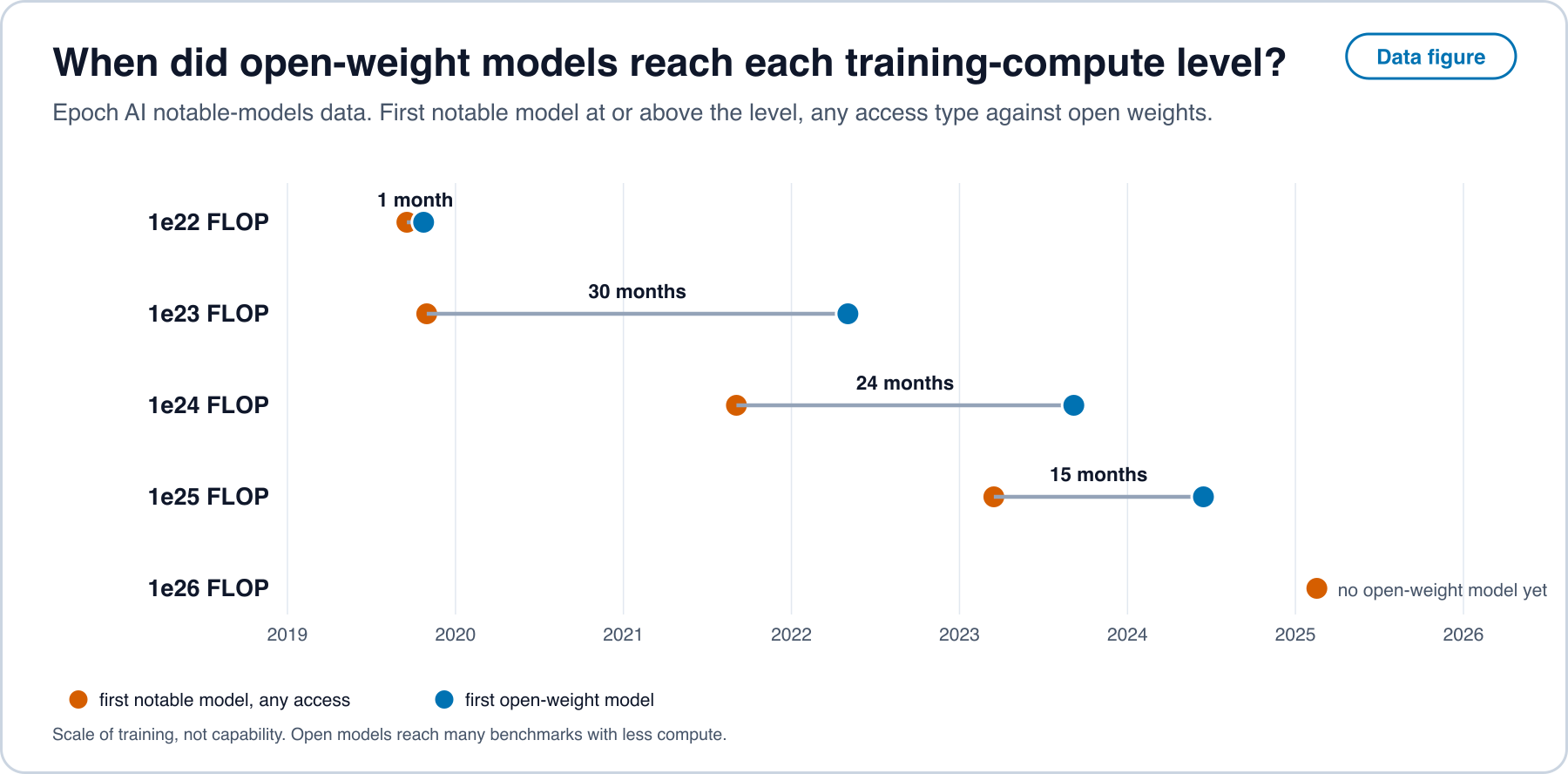
latency_data/compute_threshold_firsts.csv, from the Epoch AI notable-models dataset [25]. Open full sizeOn consumer hardware, open models that fit one consumer GPU match the frontier after an average of 6 to 12 months, depending on the measure [63]. Open-weight models of any size lag the closed frontier by about one year on benchmarks, with a range of 5 to 22 months [64].
What parity means here. It means the same benchmark score. It does not mean the same throughput: a consumer card runs one stream, and a data center serves many, where batching and kernels matter. The gains from quantization and kernels apply on both. The compute needed for a fixed performance halves about every 8 months [58], which is times a year, about twice the 1.42 times a year of hardware efficiency in Figure 11. Where that holds, algorithmic progress outruns hardware progress at a fixed quality, and parts that were bought earlier produce more tasks of a given quality than they did. Whether those extra tasks are sold at lower prices or are demanded in larger numbers is a question about demand that none of the sources here settles.
14. Other ways to build the machine
A third description is that groups making hardware by orthogonal processes show some of the cost of conventional infrastructure to be higher than the task needs. The sources read contain dated demonstrations of analog, photonic, neuromorphic, FPGA, CPU-only and flexible-electronics designs. They differ in task, scale and measurement, so this section reports each within its own paper and draws only ratios that a paper itself reports.
Table 7. Alternative designs, what was measured and the caveat.
| Approach | Demonstration | Measured or reported | Caveat |
|---|---|---|---|
| Analog in-memory | 35 million phase-change memory devices across 34 tiles on a speech keyword task [96] | Up to 12.4 TOPS per watt chip-sustained, accuracy equivalent to software | Small network, no matched baseline in the text read, so no ratio is drawn |
| Photonic | A photonic AI processor at precision the authors present as practical for ResNet and BERT [97] | Precision on those networks | No joules per task in the text read |
| Neuromorphic | A 370 million parameter MatMul-free model on Loihi 2 [28] | Up to 3 times the throughput with 2 times less energy than transformers on an edge GPU | Preliminary, small model |
| FPGA | FlightLLM on an Alveo U280 card running LLaMA2-7B with compiled sparsity and quantization [27] | 6.0 and 4.2 times the energy efficiency and 1.8 and 1.4 times the cost efficiency of a V100S and an A100 | Authors’ comparison and GPU configuration |
| Ternary weights on CPU | BitNet b1.58 2B on a CPU [26] | 0.4 GB memory against 1.4 to 4.8 GB, and 29 ms against 41 to 124 ms per token | The energy of 0.028 J per token is estimated by an arithmetic model, 6.6 to 23 times lower than the baselines, and was not read from a power meter |
| Alternative accelerator stack | Serving on Ascend NPUs [95] | 4.45 tokens per second per TFLOPS in prefill, above published H100 and H800 results | Power not reported, so no joule ratio is drawn |
| Flexible, non-silicon process | A 32-bit Arm microprocessor on a flexible substrate [98] | That a general processor can be made by a non-silicon process | No machine-learning result and no joules per task |
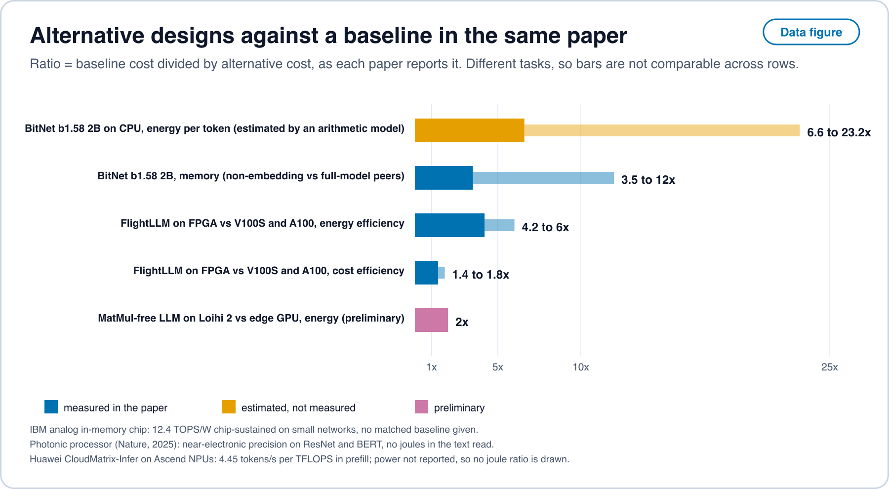
What this supports. For particular task classes, namely small models, edge deployment, CPU decoding and sparse or quantized inference on programmable logic, the authors report energy or memory 2 to 23 times lower than a conventional baseline. These are within-paper ratios on small or mid-sized models. The sources read contain no measurement of an alternative design serving a frontier-scale model, and none on wafer-scale or mature-node designs, so this article does not draw a conclusion for them.
Why an energy ratio is not a cost ratio. By Proposition 8, at data-center prices energy is between about 1.5% and 11.8% of an accelerator-hour. An alternative that lowers energy per task by a factor of 10 lowers cost per task by at most the energy share, unless it also lowers capital per task. The memory result of the ternary model points at that second path: a model that needs 0.4 GB instead of 1.4 to 4.8 GB can run on a smaller and cheaper device, and the capital effect has not been measured in the sources here. Where electricity is not the dominant term, the useful comparison is dollars per task including capital, and none of the alternative-hardware papers read reports it except FlightLLM, whose cost efficiency ratios are the smaller numbers in the table.
15. Where capability, compute and power sit
The geography of the build-out is read here from national statistics, ministries and agencies, in the original language where the source is not in English. Units differ across countries, so the figures are placed side by side and are not ranked.
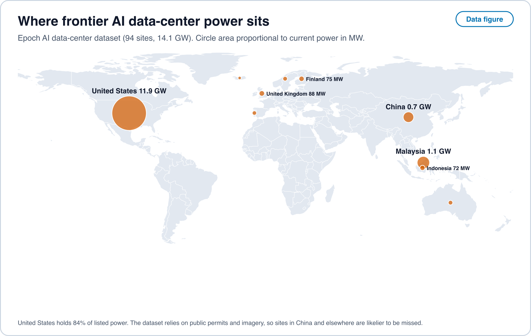
Compute and power. In the Epoch AI data-center dataset, listed frontier sites total 14.1 GW, of which the United States holds 84%, followed by Malaysia at 1.1 GW and China at 0.7 GW [12]. The dataset relies on public permits and imagery, so sites in places with less public disclosure are more likely to be missed. China’s own statistics report a different quantity: 10.85 million standard racks in use and intelligent computing capacity of 788 EFLOPS at the end of June 2025 [99], and 1.59 million PFLOPS (FP16) at the end of 2025 [100]. The two Chinese figures come from different publications and may rest on different definitions, and neither is comparable with a listed-power figure. For electricity, data centres used about 415 TWh in 2024, 1.5% of the world total, with 45% in the United States, 25% in China and 15% in Europe, and the International Energy Agency projects a doubling to about 945 TWh by 2030 as a modeled scenario [101, 102].
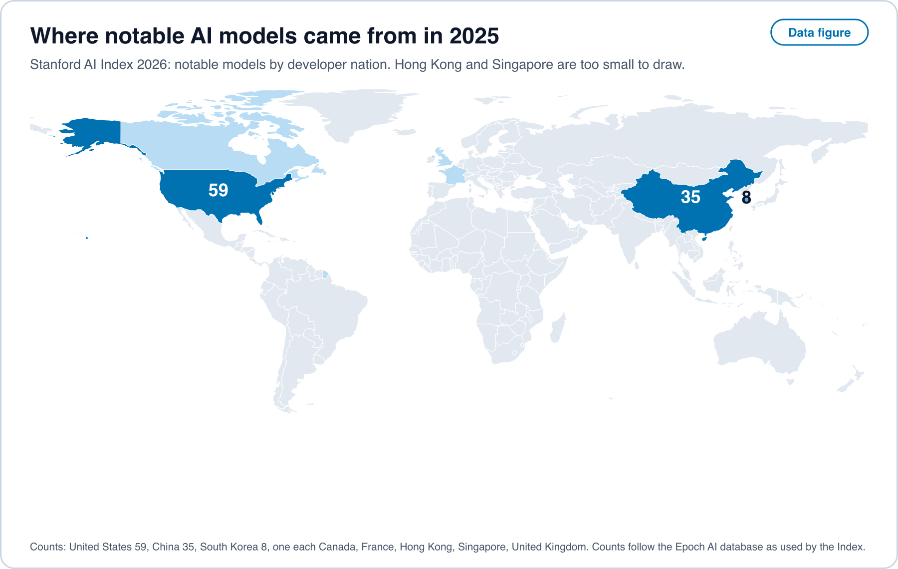
latency_data/frontier_dc_by_country.csv [12]. Open full sizeWhere models come from. Of the notable models in 2025 by national affiliation of the developer, the United States accounts for 59, China for 35 and South Korea for 8, with single models from Canada, France, Hong Kong, Singapore and the United Kingdom [29].
Chips. For the accelerators in the Epoch hardware dataset, TSMC is the recorded foundry for about four in five of the entries whose foundry is recorded, followed by Samsung, SMIC and Intel, and the foundry is not recorded for more than a third of all entries (latency_data/hardware_foundry_counts.json) [13]. The sources read gave no usable figures for packaging capacity or for fabrication capacity by country, so this article draws no map of them.
National programs. Programs state their size in different units, and Table 8 gives each as stated.
Table 8. National programs as stated, with the language of the source.
| Place | Statement | Language | Class |
|---|---|---|---|
| China | Intelligent computing capacity of 788 EFLOPS at end of June 2025 and 1.59 million PFLOPS (FP16) at end of 2025 [99, 100] | Chinese | demonstrated |
| South Korea | Government statement of securing 260,000 NVIDIA GPUs, in October 2025 [103] | Korean | opinion |
| Japan | At least 10 trillion yen of public support over the seven years to fiscal 2030, aimed at more than 50 trillion yen of private investment over ten years [104]; market research stating that cloud investment in Japanese data centers is expected to be hundreds of billions of yen or more each year [105] | Japanese | opinion |
| European Union | 200 billion euro to be mobilised for AI, with a 20 billion euro fund for AI gigafactories [106, 107] | English and Italian | opinion |
| India | 38,231 GPUs onboarded under the IndiaAI compute portal, as reported to parliament in March 2026 [108] | English | demonstrated |
| Brazil | R$ 23.03 billion of planned investment for 2024 to 2028 [109] | Portuguese | opinion |
| United Arab Emirates | A 1 GW compute cluster inside a planned 5 GW campus in Abu Dhabi [110] | English | opinion |
| Saudi Arabia | Projected capacity of up to 500 MW over five years [111] | English | opinion |
| Africa | An AI factory deploying in South Africa, with plans for Nigeria, Kenya, Egypt and Morocco; no capacity figure stated [112] | English | opinion |
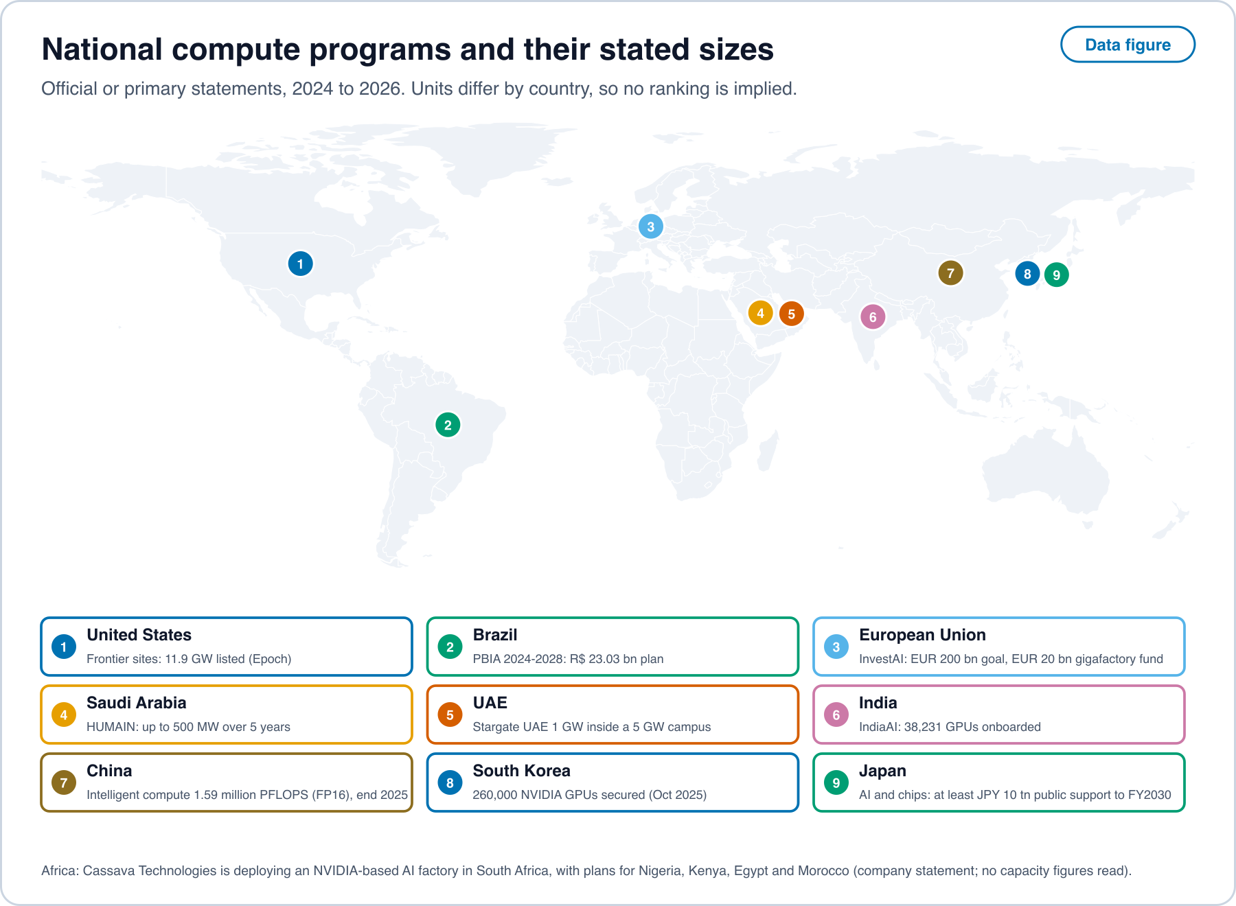
Statements in the Opinion class are plans and targets, and the Demonstrated class holds reported capacity or statistics. The two kinds should not be added.
Use. Official surveys of firms using AI give 32.9% in South Korea in 2024, 26% in Germany in 2025, 21.1% in Spain in early 2025, 20.0% in the European Union in 2025, 18% in the United States in the winter of 2025 to 2026, 13.9% for the OECD area in 2024, 13% in Brazil in 2024 and 10% in France in 2024, with years and definitions that differ [30, 31, 32, 33, 34, 35, 36, 37]. Japan and China are measured on people and not on firms [71, 72].
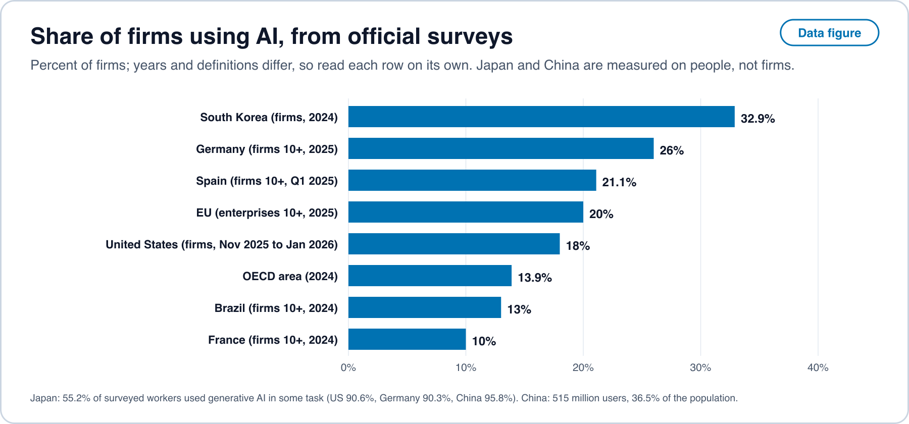
What the geography shows. Listed compute power is concentrated in one country by a wide margin, while published models and official capacity statements show a second country with a large share of models and a large stated capacity that listed-power datasets are poorly placed to see. Programs elsewhere state plans of gigawatt or hundred-billion scale, and the measured use of AI by firms is between 10% and 33% in the surveys read. The gap between plans and measured use is the gap this article studies, now at national scale.
16. Experiment protocol (not executed)
Purpose. Measure and its three parts for a list of methods, using only public dates.
Unit. A method, such as a number format, a kernel, an inference procedure or a compiler pass, with a dated public description.
Dates to collect for each method. The earliest public posting (preprint or repository), the earliest open implementation, the earliest release in a widely used open library, and the earliest general-availability release in at least one commercial product, with the firm type (listed, private, public-sector, academic). Each date is recorded with its source link and an archive copy.
Sampling. All methods in a pre-registered list drawn from a fixed set of venues and repositories over 2022 to 2026, including non-English venues and repositories, with the selection rule written before any release date is looked up.
Analysis. Compute per method. Estimate by the phase tests of Prediction 1 and by comparing the mean delay with . Estimate the gate part as the difference between listed and unlisted firms (Prediction 2). Report medians with bootstrap intervals, and report what share of methods never reach a product.
Energy. Where a method reports joules per task, record the measurement conditions, and where it does not, run it on an open energy harness such as the one cited in Table 1 and report the measured joules.
Financing and cost. Compute the bound of Definition 4 for each supplier and fiscal year from filings, the capital-loaded price of a joule from listed accelerator-hour prices and measured power, and the ratio of contracted purchases to trailing revenue for each lab, and record each with the filing and page it came from. The figure script scripts/figures/latency_figures.py and the data files under scripts/figures/latency_data/ reproduce every figure in Sections 9 to 15 from the cited sources.
Outputs. One table of dates, one analysis script, and a log of exclusions. The scripts and data are to be released with the study under the same terms as this site.
17. Conclusion
Public methods that lower the cost of computer intelligence reach products after a delay with a technical part, a calendar part and an incentive part. The first is engineering time. The second is the structure of decision dates, which on a quarterly calendar adds about six weeks on average (Proposition 1). The third appears when a reporting rule blocks a release that is worth doing in the long run (Proposition 3). A tool that lowers the cost of adopting a method removes the third once the cost falls under a stated bound, and a tool that lowers the cost of the work itself forces release when holding earns nothing (Proposition 4). When the market has several sellers reachable at low friction, the fastest sets the latency (Proposition 5). As computing cost falls, the margin that remains depends on switching friction (Proposition 6). The infrastructure evidence adds the following. Filings document loops of tens of billions of dollars between named suppliers and customers, and they bound the share of the largest chip supplier’s revenue that its own capital could have funded under a fifth, while most hyperscaler spending is paid from operating cash flow. At data-center prices energy is a small part of an accelerator-hour and capital is the large part, so cost per task follows accelerator time per task, utilization and the stated life of the machine. Open methods and alternative designs reduce accelerator time, memory or energy per task in the authors’ own measurements, for small and mid-sized models, and no source read measures them at frontier scale. Capability, compute and power are located unevenly, and national plans are stated at scales well above measured use. The propositions are a model, and the predictions name the filings, listings and measurements that would refute each.
References
Each entry ends with its evidence class (Section 1).
- Meta, joint venture with funds managed by Blue Owl Capital to develop the Hyperion data center. 2025-10-21. https://investor.atmeta.com/investor-news/press-release-details/2025/Meta-Announces-Joint-Venture-with-Funds-Managed-by-Blue-Owl-Capital-to-Develop-Hyperion-Data-Center/default.aspx (opinion)
- Meta Platforms, Quarterly Report on Form 10-Q, period ended 30 September 2025. 2025-10-30. https://www.sec.gov/Archives/edgar/data/1326801/000162828025047240/meta-20250930.htm (demonstrated)
- NVIDIA, Annual Report on Form 10-K, fiscal year ended 25 January 2026. 2026-02-25. https://www.sec.gov/Archives/edgar/data/1045810/000104581026000021/nvda-20260125.htm (demonstrated)
- CoreWeave, Annual Report on Form 10-K, fiscal year ended 31 December 2025. 2026-03-02. https://www.sec.gov/Archives/edgar/data/1769628/000176962826000104/crwv-20251231.htm (demonstrated)
- Oracle, Quarterly Report on Form 10-Q, period ended 31 August 2026. 2026-09-11. https://www.sec.gov/Archives/edgar/data/1341439/000119312626389274/orcl-20260831.htm (demonstrated)
- Oracle, Q1 FY27 results (Exhibit 99.1 to Form 8-K). 2026-09-10. https://www.sec.gov/Archives/edgar/data/1341439/000119312626387905/orcl-20260910.htm (demonstrated)
- Microsoft, Quarterly Report on Form 10-Q, period ended 30 September 2025, Note 17. 2025-10-29. https://www.sec.gov/Archives/edgar/data/789019/000119312525256321/msft-20250930.htm (demonstrated)
- OpenAI and Amazon Web Services, partnership announcement. 2025-11-03. https://openai.com/index/aws-and-openai-partnership/ (opinion)
- CNBC, OpenAI closes record-breaking 122 billion dollar funding round. 2026-03-31. https://www.cnbc.com/2026/03/31/openai-funding-round-ipo.html (opinion)
- Microsoft, NVIDIA and Anthropic, strategic partnerships announcement. 2025-11-18. https://blogs.microsoft.com/blog/2025/11/18/microsoft-nvidia-and-anthropic-announce-strategic-partnerships/ (opinion)
- U.S. Securities and Exchange Commission, XBRL company concept API (annual capital expenditure and operating cash flow, seven filers). 2026-10. https://data.sec.gov/api/xbrl/companyconcept/ (demonstrated)
- Epoch AI, Frontier Data Centers dataset (CC BY). 2026-10. https://epoch.ai/data/data-centers (demonstrated)
- Epoch AI, Machine Learning Hardware dataset (CC BY). 2026-10. https://epoch.ai/data/machine-learning-hardware (demonstrated)
- Amazon, Annual Report on Form 10-K, fiscal year ended 31 December 2025. 2026-02-06. https://www.sec.gov/Archives/edgar/data/1018724/000101872426000004/amzn-20251231.htm (demonstrated)
- Meta Platforms, Annual Report on Form 10-K, fiscal year ended 31 December 2025. 2026-01-29. https://www.sec.gov/Archives/edgar/data/1326801/000162828026003942/meta-20251231.htm (demonstrated)
- Alphabet, Annual Report on Form 10-K, fiscal year ended 31 December 2025. 2026-02-05. https://www.sec.gov/Archives/edgar/data/1652044/000165204426000018/goog-20251231.htm (demonstrated)
- Microsoft, Annual Report on Form 10-K, fiscal year ended 30 June 2026. 2026-07-29. https://www.sec.gov/Archives/edgar/data/789019/000119312626323660/msft-20260630.htm (demonstrated)
- Stanford HAI, AI Index Report 2025. 2025-04. https://hai.stanford.edu/assets/files/hai_ai_index_report_2025.pdf (demonstrated)
- Dao et al., FlashAttention: Fast and Memory-Efficient Exact Attention with IO-Awareness. 2022-05-27. https://arxiv.org/abs/2205.14135 (demonstrated)
- PyTorch, PyTorch 2.0 release announcement. 2023-03-15. https://pytorch.org/blog/pytorch-2-0-release/ (opinion)
- Gu and Dao, Mamba: Linear-Time Sequence Modeling with Selective State Spaces. 2023-12-01. https://arxiv.org/abs/2312.00752 (demonstrated)
- Lieber et al., Jamba: A Hybrid Transformer-Mamba Language Model. 2024-03-28. https://arxiv.org/abs/2403.19887 (demonstrated)
- Leviathan, Kalman, Matias, Fast Inference from Transformers via Speculative Decoding. 2022-11-30 (ICML 2023). https://arxiv.org/abs/2211.17192 (established by proof in the source)
- Google Research, Looking back at speculative decoding. 2024-12-06. https://research.google/blog/looking-back-at-speculative-decoding/ (opinion)
- Epoch AI, Notable AI Models dataset (CC BY). 2026-10. https://epoch.ai/data/notable-ai-models (demonstrated)
- Ma et al., BitNet b1.58 2B4T Technical Report. 2025-04-16. https://arxiv.org/abs/2504.12285 (demonstrated)
- Zeng et al., FlightLLM: Efficient Large Language Model Inference with a Complete Mapping Flow on FPGAs. 2024-01-08. https://arxiv.org/abs/2401.03868 (demonstrated)
- Abreu et al., Neuromorphic Principles for Efficient Large Language Models on Intel Loihi 2. 2025-03. https://arxiv.org/abs/2503.18002 (demonstrated)
- Stanford HAI, AI Index Report 2026, research and development chapter. 2026-04. https://hai.stanford.edu/ai-index/2026-ai-index-report (demonstrated)
- (Korean) Electronic Times, reporting the 2025 Enterprise Informatization Statistics of the Ministry of Science and ICT and NIA. 2026-01-20. https://www.etnews.com/20260120000071 (demonstrated)
- (German) Statistisches Bundesamt, Unternehmen mit Nutzung von Technologien der künstlichen Intelligenz nach Beschäftigtengrößenklassen (table, 2025). 2025. https://www.destatis.de/DE/Themen/Branchen-Unternehmen/Unternehmen/IKT-in-Unternehmen-IKT-Branche/Tabellen/ikti-unternehmen-kuenstliche-intelligenz.html (demonstrated)
- (Spanish) Instituto Nacional de Estadística, Encuesta sobre el uso de TIC y del comercio electrónico en las empresas, nota de prensa. 2025-10-22. https://ine.es/dyngs/Prensa/ETICCE20241T2025.pdf (demonstrated)
- Eurostat, 20% of EU enterprises use AI technologies. 2025-12-11. https://ec.europa.eu/eurostat/documents/7870049/23260410/KS-01-26-009-EN-N.pdf (demonstrated)
- Bonney et al., The Microstructure of AI Diffusion (Census CES-WP-26-25). 2026-04. https://www.census.gov/library/working-papers/2026/adrm/CES-WP-26-25.html (demonstrated)
- OECD, Emerging divides in the transition to artificial intelligence. 2025-06. https://www.oecd.org/content/dam/oecd/en/publications/reports/2025/06/emerging-divides-in-the-transition-to-artificial-intelligence_eeb5e120/7376c776-en.pdf (demonstrated)
- (Portuguese) Cetic.br/NIC.br, Pesquisa TIC Empresas 2024, resumo executivo. 2025-05. https://www.nic.br/media/docs/publicacoes/2/20250512121759/tic_empresas_2024_resumo_executivo.pdf (demonstrated)
- (French) Insee, Les technologies de l’information et de la communication dans les entreprises en 2024, Insee Première n° 2061. 2025-07. https://www.insee.fr/fr/statistiques/fichier/8604126/ip2061.pdf (demonstrated)
- Dao and Gu, Transformers are SSMs (Mamba-2, state space duality). 2024-05-31. https://arxiv.org/abs/2405.21060 (established by proof in the source)
- Lieber et al. (Jamba); NVIDIA (Nemotron-H); TII (Falcon-H1); IBM (Granite 4.0). 2024 to 2025. https://arxiv.org/abs/2504.03624 (demonstrated)
- Ma et al., The Era of 1-bit LLMs (BitNet b1.58). 2024-02-27. https://arxiv.org/abs/2402.17764 (demonstrated)
- NVIDIA, Pretraining Large Language Models with NVFP4. 2025-09. https://arxiv.org/abs/2509.25149 (demonstrated)
- Shah et al., FlashAttention-3. 2024-07. https://arxiv.org/abs/2407.08608 (demonstrated)
- Yuan et al., Native Sparse Attention. 2025-02 (ACL 2025). https://arxiv.org/abs/2502.11089 (demonstrated)
- Hoffmann et al., Training Compute-Optimal Large Language Models. 2022-03-29. https://arxiv.org/abs/2203.15556 (demonstrated)
- Sardana et al., Beyond Chinchilla-Optimal: Accounting for Inference in Language Model Scaling. 2024-01 (ICML 2024). https://arxiv.org/abs/2401.00448 (demonstrated)
- DeepSeek-AI, DeepSeek-V3 Technical Report. 2024-12-26. https://arxiv.org/abs/2412.19437 (demonstrated)
- Angelopoulos, Barber, Bates, Theoretical Foundations of Conformal Prediction. 2024-11-18 (v5 2026-03-06). https://arxiv.org/abs/2411.11824 (established by proof in the source)
- Zhou, Chen, Gui and Cheng, Conformal Prediction: A Data Perspective. 2024-10 (arXiv 2410.06494; ACM Computing Surveys 2025). https://arxiv.org/abs/2410.06494 (opinion)
- Angelopoulos et al., Prediction-powered inference. 2023 (Science). https://www.science.org/doi/10.1126/science.adi6000 (established by proof in the source)
- Ramdas, Grunwald, Vovk, Shafer, Game-Theoretic Statistics and Safe Anytime-Valid Inference. 2023-11 (Statistical Science 38(4)). https://doi.org/10.1214/23-sts894 (established by proof in the source)
- Chernozhukov et al., Double/debiased machine learning. 2018 (Econometrics Journal). https://doi.org/10.1111/ectj.12097 (established by proof in the source)
- Jung, Tian, Bareinboim, Estimating Identifiable Causal Effects through Double Machine Learning. 2021 (AAAI). https://doi.org/10.1609/aaai.v35i13.17438 (established by proof in the source)
- Sathia et al., Compiler Optimizations for Higher-Order Automatic Differentiation. 2025 (PPoPP workshop). https://ece.is/assets/pdf/diffprog-ppopp25-paper90.pdf (demonstrated)
- Ward et al., JAX a la Stan. 2026-10-11. https://bob-carpenter.github.io/dj-paper/template-computo-python.pdf (opinion)
- Qian et al., Impulse: probabilistic programming via compiler augmentation. 2026 (abstract). https://ece.is/assets/pdf/impulse-pldi-src-abstract.pdf (demonstrated)
- Chung et al., The ML.ENERGY Benchmark. 2025 (NeurIPS Datasets and Benchmarks). https://ml.energy/leaderboard/ (demonstrated)
- Google, Measuring the environmental impact of delivering AI at Google Scale. 2025-08. https://arxiv.org/abs/2508.15734 (demonstrated)
- Ho et al. (Epoch AI), Algorithmic progress in language models. 2024-03 (NeurIPS 2024). https://arxiv.org/abs/2403.05812 (demonstrated)
- Epoch AI, LLM inference prices have fallen rapidly but unequally across tasks. 2025. https://epoch.ai/data-insights/llm-inference-price-trends (demonstrated)
- Comin and Hobijn, An Exploration of Technology Diffusion. 2010 (AER 100(5)). https://doi.org/10.1257/aer.100.5.2031 (demonstrated)
- P. A. David, The Dynamo and the Computer. 1990 (AER 80(2)). https://ideas.repec.org/a/aea/aecrev/v80y1990i2p355-61.html (demonstrated)
- Brynjolfsson, Rock, Syverson, The Productivity J-Curve. 2021 (AEJ Macro). https://doi.org/10.1257/mac.20180386 (demonstrated)
- Somala and Emberson (Epoch AI), Frontier AI performance becomes accessible on consumer hardware within a year. 2025-08-15. https://epoch.ai/data-insights/consumer-gpu-model-gap (demonstrated)
- Epoch AI, Open vs. closed AI: how behind are open models?. 2025. https://epoch.ai/publications/open-models-report (demonstrated)
- Gupta and Kiely, Production-ready speculative decoding with TensorRT-LLM. 2024-12-19. https://www.baseten.co/blog/how-we-built-production-ready-speculative-decoding-with-tensorrt-llm/ (opinion)
- Marx and Fuegi, Reliance on Science: Worldwide Front-Page Patent Citations to Scientific Articles. 2020 (NBER 27987; JEMS 2022). https://www.nber.org/system/files/working_papers/w27987/w27987.pdf (demonstrated)
- Ahmadpoor and Jones, The dual frontier. 2017 (Science). https://doi.org/10.1126/science.aam9527 (demonstrated)
- Willison, Stanford Alpaca, and the acceleration of on-device large language model development. 2023-03-13. https://simonwillison.net/2023/Mar/13/alpaca/ (opinion)
- Li et al., Now Hiring: Firm-Level Adoption of Generative AI in China (World Bank). 2025/2026. https://thedocs.worldbank.org/en/doc/cbdef4ef57efdbb3c29aa4c07edf860b-0050062026/original/Now-hiring-Firm-Level-Li-etal.pdf (demonstrated)
- (German) Statistisches Bundesamt, Pressemitteilung Nr. 444: Jedes fünfte Unternehmen nutzt künstliche Intelligenz. 2024-11-25. https://www.destatis.de/DE/Presse/Pressemitteilungen/2024/11/PD24_444_52911.html (demonstrated)
- Japan Ministry of Internal Affairs and Communications, 令和7年版情報通信白書 (Information and Communications White Paper 2025), data tables, in Japanese. 2025. https://www.soumu.go.jp/johotsusintokei/whitepaper/ja/r07/html/nd112220.html (demonstrated)
- (Chinese) China Internet Network Information Center, 生成式人工智能应用发展报告(2025). 2025-10. https://pdf.dfcfw.com/pdf/H301_AP202510241768289458_1.pdf (demonstrated)
- Bick, Blandin, Deming, The Rapid Adoption of Generative AI. 2024-09 (rev. 2025-02). https://www.nber.org/papers/w32966 (demonstrated)
- Brynjolfsson, Li, Raymond, Generative AI at Work (NBER Working Paper 31161; later published in QJE 2025). 2023 working paper, revised. https://www.nber.org/papers/w31161 (demonstrated)
- METR, Measuring the Impact of Early-2025 AI on Experienced Open-Source Developer Productivity. 2025-07-10. https://arxiv.org/abs/2507.09089 (demonstrated)
- Bloom, Jones, Van Reenen, Webb, Are Ideas Getting Harder to Find?. 2020 (AER 110(4)). https://doi.org/10.1257/aer.20180338 (demonstrated)
- Graham, Harvey, Rajgopal, The Economic Implications of Corporate Financial Reporting. 2005 (JAE 40); NBER 2004-10. https://www.nber.org/papers/w10550 (demonstrated)
- Asker, Farre-Mensa, Ljungqvist, Corporate Investment and Stock Market Listing: A Puzzle?. 2015 (RFS 28(2)). https://doi.org/10.1093/rfs/hhu077 (demonstrated)
- FactSet, Highest number of S&P 500 earnings calls citing AI over the past 10 years. 2025-12. https://insight.factset.com/highest-number-of-sp-500-earnings-calls-citing-ai-over-the-past-10-years-1 (demonstrated)
- Hassan, Hollander, van Lent, Tahoun, Firm-Level Political Risk. 2019 (QJE 134(4)). https://doi.org/10.1093/qje/qjz021 (demonstrated)
- Metrick and Yasuda, Venture Capital and Other Private Equity: A Survey (NBER Working Paper 16652). 2010-10. https://www.nber.org/system/files/working_papers/w16652/w16652.pdf (opinion)
- Gompers and Lerner, What Drives Venture Capital Fundraising? (Brookings Papers: Microeconomics). 1998. https://www.brookings.edu/wp-content/uploads/1998/01/1998_bpeamicro_gompers.pdf (demonstrated)
- Arrow, Economic Welfare and the Allocation of Resources for Invention (NBER chapter). 1962. https://www.nber.org/system/files/chapters/c2144/c2144.pdf (established by proof in the source)
- Shapiro, Competition and Innovation: Did Arrow Hit the Bull’s Eye? (NBER conference draft). 2010. https://conference.nber.org/confer/2010/RDIA10/Shapiro.pdf (opinion)
- Henderson and Clark, Architectural Innovation. 1990 (ASQ 35(1)). https://doi.org/10.2307/2393549 (demonstrated)
- US District Court for D.C., United States v. Google LLC, remedies memorandum. 2025-09-02. https://www.courthousenews.com/wp-content/uploads/2025/09/judge-amit-mehta-google-search-monopoly-remedy-ruling.pdf (demonstrated)
- NVIDIA and OpenAI, letter of intent announcement. 2025-09-22. https://nvidianews.nvidia.com/news/openai-and-nvidia-announce-strategic-partnership-to-deploy-10gw-of-nvidia-systems (opinion)
- Advanced Micro Devices, Form 8-K, Item 1.01 (warrant issued to OpenAI). 2025-10-06. https://www.sec.gov/Archives/edgar/data/2488/000119312525230895/d28189d8k.htm (demonstrated)
- Microsoft, The next chapter of the Microsoft-OpenAI partnership. 2025-10-28. https://blogs.microsoft.com/blog/2025/10/28/the-next-chapter-of-the-microsoft-openai-partnership/ (opinion)
- Anthropic, Expanding our use of Google Cloud TPUs and services. 2025-10-23. https://www.anthropic.com/news/expanding-our-use-of-google-cloud-tpus-and-services (opinion)
- OpenAI and Broadcom, strategic collaboration announcement. 2025-10-13. https://openai.com/index/openai-and-broadcom-announce-strategic-collaboration/ (opinion)
- Frantar et al., GPTQ: Accurate Post-Training Quantization for Generative Pre-trained Transformers. 2022-10-31. https://arxiv.org/abs/2210.17323 (demonstrated)
- Kwon et al., Efficient Memory Management for Large Language Model Serving with PagedAttention (vLLM). 2023-09-12. https://arxiv.org/abs/2309.06180 (demonstrated)
- DeepSeek-AI, DeepSeek-R1: Incentivizing Reasoning Capability in LLMs via Reinforcement Learning. 2025-01-22. https://arxiv.org/abs/2501.12948 (demonstrated)
- Zuo et al., Serving Large Language Models on Huawei CloudMatrix384. 2025-06. https://arxiv.org/abs/2506.12708 (demonstrated)
- Le Gallo et al., An analog-AI chip for energy-efficient speech recognition and transcription, Nature. 2023-08-23. https://www.nature.com/articles/s41586-023-06337-5 (demonstrated)
- Ahmed et al., Universal photonic artificial intelligence acceleration, Nature. 2025-04-09. https://www.nature.com/articles/s41586-025-08854-x (demonstrated)
- Biggs et al., A natively flexible 32-bit Arm microprocessor, Nature. 2021-07-21. https://www.nature.com/articles/s41586-021-03625-w (demonstrated)
- (Chinese) 国务院, 截至今年6月底我国智能算力规模达788百亿亿次/秒 (人民日报). 2025-09-02. https://www.gov.cn/yaowen/liebiao/202509/content_7038732.htm (demonstrated)
- (Chinese) 全国数据资源统计调查工作组, 全国数据资源调查报告(2025年). 2026. https://www.nda.gov.cn/sjj/swdt/xwfb/0429/ff808081-9b5e8626-019d-d86b2f54-1154.pdf (demonstrated)
- International Energy Agency, Energy and AI, executive summary. 2025-04. https://www.iea.org/reports/energy-and-ai/executive-summary (demonstrated)
- International Energy Agency, Energy and AI, energy demand from AI. 2025-04. https://www.iea.org/reports/energy-and-ai/energy-demand-from-ai (demonstrated)
- (Korean) 뉴시스, 정부, 엔비디아 GPU 26만장 확보. 2025-10-31. https://www.newsis.com/view/NISX20251031_0003385059 (opinion)
- (Japanese) 経済産業省, AI・半導体産業基盤強化フレーム. 2024-11. https://www.meti.go.jp/policy/mono_info_service/ai_semiconductor_frame/ai_semiconductor_frame.html (opinion)
- (Japanese) 総務省 有識者会合 資料5, 国内データセンター市場におけるAI需要・地方分散・再エネ電源 (富士キメラ総研). 2024-05-30. https://www.meti.go.jp/policy/mono_info_service/joho/conference/digital_infrastructure/0007/005_fujichimera.pdf (opinion)
- European Commission, EU launches InvestAI initiative to mobilise 200 billion euro (English). 2025-02-11. https://digital-strategy.ec.europa.eu/en/news/eu-launches-investai-initiative-mobilise-eu200-billion-investment-artificial-intelligence (opinion)
- (Italian) Commissione europea, UE lancia InvestAI per mobilitare 200 miliardi di EUR. 2025-02-11. https://digital-strategy.ec.europa.eu/it/news/eu-launches-investai-initiative-mobilise-eu200-billion-investment-artificial-intelligence (opinion)
- Press Information Bureau (India), reply in the Lok Sabha on the IndiaAI Mission. 2026-03-25. https://www.pib.gov.in/PressReleasePage.aspx?PRID=2245063 (demonstrated)
- (Portuguese) Ministério da Ciência, Tecnologia e Inovação, Plano Brasileiro de Inteligência Artificial 2024-2028. 2025. https://www.gov.br/mcti/pt-br/acompanhe-o-mcti/transformacaodigital/plano-brasileiro-de-inteligencia-artificial (opinion)
- SoftBank Group, Global Tech Alliance Launches Stargate UAE. 2025-05-22. https://group.softbank/en/news/press/20250522 (opinion)
- NVIDIA, HUMAIN and NVIDIA Announce Strategic Partnership to Build AI Factories in Saudi Arabia. 2025-05-13. https://nvidianews.nvidia.com/news/humain-and-nvidia-announce-strategic-partnership-to-build-ai-factories-of-the-future-in-saudi-arabia (opinion)
- Cassava Technologies, Cassava scales African AI infrastructure with NVIDIA-powered AI factories. 2025. https://www.cassavatechnologies.com/cassava-scales-african-ai-infrastructure-with-nvidia-powered-ai-factories-to-accelerate-sovereign-data-capabilities/ (opinion)